A Hybrid Soft Computing Model to Predict Time-to-break Margins in

When will it break? A Hybrid Soft Computing Model to Predict Time-to-break Margins in Paper Machines Piero P. Bonissone and Kai Goebel General Electric Global Research Center Schenectady, NY 12309, USA ABSTRACT Hybrid soft computing models, based by neural, fuzzy and evolutionary computation technologies, have been applied to a large number of classification, prediction, and control problems. This paper focuses on one of such applications and presents a systematic process for building a predictive model to estimate time-to-breakage and provide a web break tendency indicator in the wet-end part of paper making machines. Through successive information refinement of information gleaned from sensor readings via data analysis, principal component analysis (PCA), adaptive neural fuzzy inference system (ANFIS), and trending analysis, a break tendency indicator was built. Output of this indicator is the break margin. The break margin is then interpreted using a stoplight metaphor. This interpretation provides a more gradual web break sensitivity indicator, since it uses more classes compared to a binary indicator. By generating an accurate web break tendency indicator with enough leadtime, we help in the overall control of the paper making cycle by minimizing down time and improving productivity. Keywords: Soft Computing, ANFIS, Principal Components, Paper Industry Application.

1. INTRODUCTION 1.1 Soft Computing Soft Computing (SC), sometimes also referred to as Computational Intelligence, was originally defined by Zadeh (1994) as an association of computing methodologies that “…exploit the tolerance for imprecision, uncertainty, and partial truth to achieve tractability, robustness, low solution cost, and better rapport with reality.” According to Zadeh (1998), Soft Computing “includes as its principal members fuzzy logics (FL), neuro-computing (NC), evolutionary computing (EC) and probabilistic computing (PC).” As we remarked in reference (Bonissone 2001b), the main reason for the popularity of soft computing is the synergy derived from its components. In fact, SC’s main characteristic is its intrinsic capability to create hybrid systems that are based on the integration of constituent technologies. This integration provides complementary reasoning and searching methods that allow us to combine domain knowledge and empirical data to develop flexible computing tools and solve complex problems. Soft Computing provides a different paradigm in terms of representation and methodologies, which facilitates these integration attempts. For instance, in classical control theory the problem of developing models is usually decomposed into system identification (or system structure) and parameter estimation. The former determines the order of the differential equations, while the latter determines its coefficients. In these traditional approaches, the main goal is the construction of accurate models, within the assumptions used for the model construction. However, the models’ interpretability is very limited, given the rigidity of the underlying representation language. The equation “model = structure + parameters”, followed by the traditional approaches to model building, does not change with the advent of soft computing. However, with soft computing we have a much richer repertoire to represent the structure, to tune the parameters, and to iterate this process. This repertoire enables us to choose among different tradeoffs between the model’s interpretability and accuracy. For instance, one approach aimed at maintaining the model’s transparency might start with knowledge-derived linguistic models, where the domain knowledge is translated into an initial structure and parameters. Then the model’s accuracy could be improved by using global or local data-driven search methods to tune the structure and/or the parameters. An alternative approach aimed at building more accurate models might start with data-driven search methods. Then, we could embed domain knowledge into the search operators to control or limit the search space, or to maintain the model’s interpretability. Post-processing approaches could also be used to extract more explicit structural information from the models. Extensive coverage of SC components can be found in Back et al. (1997), Fiesler and Beale (1997) and Ruspini et al. (1998). Hybrid SC systems are further described in Bonissone (1997), and Bonissone et al. (1999b).

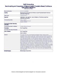
1.2 Problem Description The problem under study is the breakage of the paper web in a paper-making machine at the wet end, specifically at or near the site of the center roll (Chen and Bonissone, 1998). A schematic of a paper machine is depicted in Figure 1. Web breaks typically result in a loss of 5-12% of production, with rather big impact on revenue. The paper mill considered had an average of 35 wet-end breaks every month on a machine, with a peak value of as much as 15 in a single day. The average production time lost as a result of these breaks is 1.6 hours/day. Considering that each paper machine works continuously (24 hours a day, every day of the year), this downtime translates to 1.6/24 = 6.66% of its annual production. Given the paper industry’s installed basis of hundreds of paper machines, producing worldwide revenues of about $45 billions, this translates to loss revenue of $3 billions every year. Dry-end breaks are relatively well understood, while wet-end breaks are harder to explain in terms of causes and are harder to predict and control. This has to do in part with the time it takes to process the paper material starting from the pulp until it ends up as paper on the final roll versus the warning limits. The latter are considerably longer than the paper processing time. That means that a prognostics system can only deal with system changes that have long transients such as material build-up on drums, etc. It means also that the prognostics has relatively little opportunity to react to material variability because there is by design not enough time to warn against breaks related to these conditions. The aim of this project is to design a web break predictor that will address to predict system changes leading to breaks at the wet-end (Bonissone et al., 1999a, Chen and Bonissone 2002). This predictor will also output margin of breaks, i.e., how much time left to a web break. This will help engineers to better anticipate the breaks and take remedial action. Specific requirements were to issue the warning at least 60 minutes before the breakage and potentially up to 90 minutes prior to the breakage. In addition, high priority was placed on avoiding false positive warnings. Paper machine Pulp Water

Wet-end

Press section

Dry-end

Paper

Water

Figure 1. Schematic of a paper machine.

The problem to be solved, then, is the design of a robust model to predict the break tendency and time-to-breakage of the paper web in a paper making machine at the wet end (specifically at or near the site of the center roll). We report here about the proposed solution that is the result of a development process covering several years. In the course of this process, numerous techniques were evaluated and – if they contributed to an improvement of the outcome – incorporated into the solution. The resulting information refinement process involved data analysis (identification of relevant variables, extraction of structure information from data via models, model development based on machine learning techniques, and creation of a break tendency and a time-to-breakage predictors), prototype algorithm development, and validation of the predictive model with test data. We feel this prognostic process is not only applicable for wet-end time-to-breakage prediction but also applicable to other proactive diagnostics problems in the service arena and in fact we conducted successful pilot studies in other domains such as predicting failure for certain failure modes of magnets in magnetic resonance imaging (MRI) equipment. Data Reduction 2 Data Data segmentation scrubbing

Variable 3 Reduction 4 Variable PCA selection

1

Model Generation 7 8 NormaliTransformzation ation

9 Shuffling

10 ANFI S

11 Trending

Value 6 5 Transformations Filtering Smoothing

Time to Breakage Prediction

Figure 2: Overview of prognostics process

Break Indicator

12 Performance Evaluation

An overview of the system is schematically represented in Figure 2. There are two modes for the system—training and testing modes. In the training mode, historical web breaks data gathered by sensors are acquired and analyzed, signal processing techniques are applied, and an ANFIS model is fitted to the data off-line. In the testing mode, the sensor readings are analyzed first using the same techniques as in the training phase (except in run-time mode). Next, the ANFIS model takes as input the preprocessed sensor data and gives as output the prediction of time-to-breakage on the fly. This model is used to drive a stoplight display, in which the yellow and red lights represent a 90-minute and 60-minute alarm, respectively. 1.3 Structure of paper In the second section we will describe our proposed multistage process, and we will illustrate the steps in data reduction, variable selection, value transformation, model generation, time-to-break prediction, and break indicator. In the third section we will present the prediction results for the training and validation sets. The last section will contain our concluding remarks and possible future work.

2. SOLUTION DESCRIPTION 2.1 Data Reduction The first activity of our model building process was Data Reduction. Its main purpose was to render the original data suitable for model building purpose. Data were collected during the time period from June 1999 to February 2000. These data needed to be scrubbed and reduced, in order to be used to build predictive models. Observations needed to be organized as time-series or break trajectories. The scope of this project was limited to the prediction of breaks with unknown causes, so we only considered break trajectories associated with unknown causes and eliminated other break trajectories. We needed to separate the trajectories containing a break or recorded in a 180-minute window prior to the break from the ones recorded before such window. Since these two groups formed the basis for the supervised training of our models, we needed to label them accordingly. Most data obtained from sensor readings exhibit some incorrect observations - with missing or zero values recorded for long period of time. These were removed. We did not remove paper grade variability for this particular machine, which was assumed not to cause big variations. This was confirmed upon inspection by an expert team. However, in general, paper grade changes can cause significant changes in process variables and can also be the cause of wet-end breakage. The activity was then subdivided into two steps, labeled “Data Scrubbing” (step 1) and “Data Segmentation” (step 2), which are described below. Step 1. Data Scrubbing. We grouped the data according to various break trajectories. A break trajectory is defined as a multivariate time-series starting at a normal operating condition and ending at a wet-end break. A long break trajectory could last up to a couple of days, while a short break trajectory could be less than three hours long. We started with roughly 88 break trajectories and 43 variables. Data were grouped according to various break trajectories, namely known break causes and unknown break causes. It was only interesting to consider breaks that could potentially be prevented. This excluded breaks that had known causes such as extremely rare chance events (“observed grease like substance falling on web”), grade changes, machine operation changes, or other non-process failures. After that, we extracted both break negative and positive data from this group. Finally, we deleted incomplete observations and obviously missing values. This resulted in a set of 41 break trajectories. Step 2. Data Segmentation. After the data scrubbing process, we segmented the data sets into two parts. The first one contained the set of observations taken at the moment of a break and no less than 180 minutes prior to each break. For example, there were a number of breaks occurring in quick succession (break avalanches) which were not suitable for break prediction purposes. Other trajectories contained not the required number of data for other reasons. The resulting remaining data set was denoted as Break Positive Data (BPD). Trajectories that extended beyond 180 minutes were considered to be in steady state (for breakage purposes) and denoted as Break Negative Data (BND). After the data scrubbing and data segmentation, we had break positive data that consisted of 25 break trajectories. 2.2 Variable Reduction The second activity of our model building process was Variable Reduction. Its main purpose was to derive the simplest possible model that could explain the past (training mode) and predict the future (testing mode). Typically, the complexity of a model increases in a nonlinear way with the number of inputs used by the model. High complexity models tend to be excellent in training mode but rather brittle in testing mode. Usually, these models tend to overfit the training data and do not generalize well to new situations - we will refer to this as lack of model robustness. Therefore, a reduction in the number of variables (by a combination of variable selection and variable composition) and its associated reduction of inputs enabled us

to derive simpler, more robust models. This activity was subdivided into two steps, labeled Variable Selection (step 3), and Principal Component Analysis (step 4), which are described below. Step 3. Variable Selection. In the presence of noise it is desirable to use as few variables as possible, while predicting well. This is often referred as “principle of parsimonious.” There may be combinations (linear or nonlinear) of variables that are actually irrelevant to the underlying process, that due to noise in data appear to increase the prediction accuracy. The idea is to use combinations of various techniques to select the variables with the greater discrimination power in break prediction. It is a modeling bias in favor of smaller models, to trade the potential ability to discover better fitting models with protection from overfitting, i.e., “inventing features when there are none” (Ali and Wallace, 1993). From the implementation point of view the risk of more variables in the model is not limited to the danger of overfitting. It also involves the risk of more sensors malfunctioning and misleading the model predictions. In an academic setting, the risk return tradeoff may be more tilted toward risk taking for higher potential accuracy. Out of 41 potential sensor readings, we dropped a total of 21 in a joint review with experts knowledgeable of the process due to the sensors’ apparent information content for the prediction problem.

2.55

PC1

2.75

Step 4. Principal Components Analysis (PCA). A principal components analysis (PCA) is concerned with explaining the variance-covariance structure through a few linear combinations of the original variables (Johnson and Wichern, 1988). Its general objectives are data reduction and data interpretation. Although p components are required to reproduce the total system variability, often much of this variability can be accounted for by a smaller number k of the principal components (k