Sung K. Koh Department of Mechanical Engineering, Pohang University of Science and Technology, Pohang, 790-784, Republic of Korea e-mail:
[email protected]
Gregory S. Chirikjian Department of Mechanical Engineering, Johns Hopkins University, Baltimore, MD 21218 e-mail:
[email protected]
G. K. Ananthasuresh Department of Mechanical Engineering, Indian Institute of Science, Bangalore, 560012, India e-mail:
[email protected]
A Jacobian-Based Algorithm for Planning Attitude Maneuvers Using Forward and Reverse Rotations Algorithms for planning quasistatic attitude maneuvers based on the Jacobian of the forward kinematic mapping of fully-reversed (FR) sequences of rotations are proposed in this paper. An FR sequence of rotations is a series of finite rotations that consists of initial rotations about the axes of a body-fixed coordinate frame and subsequent rotations that undo these initial rotations. Unlike the Jacobian of conventional systems such as a robot manipulator, the Jacobian of the system manipulated through FR rotations is a null matrix at the identity, which leads to a total breakdown of the traditional Jacobian formulation. Therefore, the Jacobian algorithm is reformulated and implemented so as to synthesize an FR sequence for a desired rotational displacement. The Jacobian-based algorithm presented in this paper identifies particular six-rotation FR sequences that synthesize desired orientations. We developed the single-step and the multiple-step Jacobian methods to accomplish a given task using six-rotation FR sequences. The single-step Jacobian method identifies a specific FR sequence for a given desired orientation and the multiple-step Jacobian algorithm synthesizes physically feasible FR rotations on an optimal path. A comparison with existing algorithms verifies the fast convergence ability of the Jacobian-based algorithm. Unlike closed-form solutions to the inverse kinematics problem, the Jacobian-based algorithm determines the most efficient FR sequence that yields a desired rotational displacement through a simple and inexpensive numerical calculation. The procedure presented here is useful for those motion planning problems wherein the Jacobian is singular or null. 关DOI: 10.1115/1.3007903兴 Keywords: attitude control, fully-reversed sequences of rotations, noncommutativity of finite rigid rotations, Jacobian algorithm, inverse kinematics, motion planning
1
Introduction
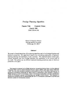
A Jacobian-based algorithm to specify the orientation of a free rigid body undergoing fully-reversed 共FR兲 sequences of rotations is presented in this paper. An FR sequence of rotations is defined as a series of rotations that consists of a series of initial forward rotations about the axes of a coordinate frame attached to a rigid body and a series of subsequent rotations that reverse the preceding forward rotations 关1–4兴. Since finite rotations of a rigid body are not commutative, finite FR rotations lead to a net orientation change of the rigid body. The non-commutative property of finite rigid rotations is illustrated in Fig. 1. The cube in Fig. 1 undergoes successive rotations of 90 deg about the axes x, y, z, −x, −y, and −z. The orientation of the cube at the end of this fully-reversed operation is not the same as its initial orientation. We exploit six-rotation FR sequences of rotations to achieve a net orientation change of a rigid body because six-rotation FR sequence has sufficient degrees of freedom that are required to synthesize any possible orientations of the rigid body. Six-rotation FR sequences are composed of three initial forward rotations and three subsequent rotations in the reverse directions. The FR operation shown in Fig. 1 is an example of a six-rotation FR sequence. In this paper, we are concerned with Contributed by the Design Engineering Division for publication in the JOURNAL OF COMPUTATIONAL AND NONLINEAR DYNAMICS. Manuscript received June 18, 2007; final manuscript received May 20, 2008; published online December 12, 2008. Review conducted by Olivier A. Bauchau. Paper presented at the ASME 2007 Design Engineering Technical Conferences and Computers and Information in Engineering Conference 共DETC2007兲, Las Vegas, NV, September 4–7, 2007.
planning a correct FR sequence to re-orient the body to a desired orientation. The dynamics of the rigid body is beyond the scope of this paper. The need for FR sequences of rotations stems from the working principle of the micro-scale device of Fig. 2共b兲 developed for quasistatic orientation control of a spacecraft. Li et al. 关1兴 proposed a microscale pseudo-momentum-wheel as an alternative to the conventional torque generation mechanisms of spacecraft. The pseudo-momentum-wheel shown in Fig. 2共b兲 is an array of radially projecting microscale electro-thermal-compliant 共ETC兲 actuators and generates a torque from the elastic deformation of its U-shape structure, as shown in Fig. 2共c兲. Upon application of a voltage to the ETC actuator, non-uniform temperature distribution on the actuator caused by Joule heating effects leads it to bend, as shown in Fig. 2共c兲. Therefore, when the pseudo-wheels are mounted on the surface of a rigid-cube, as shown in Fig. 2共a兲, the activation of the pseudo-wheel produces a torque to conserve the angular momentum of the system. However, when the actuators are deactivated quasistatically, they recover their original undeformed shape, which causes reverse directional rotations following the initial forward rotations. Therefore, the reverse rotations are inevitable when the rigid-cube is maneuvered by ETC pseudowheels. This provides the motivation for studying the kinematics of a rigid body that reorients its orientation through fully-reversed rotations according to the non-commutativity of finite rotations. According to the experiments with prototype pseudo-wheels 关1兴, it takes about the order of milliseconds for the activation and deactivation of the ETC actuators. Therefore, we assume that the time required to turn on and off the ETC actuators is 1 ms throughout the examples presented in this paper. Since the moment of inertia
Journal of Computational and Nonlinear Dynamics Copyright © 2009 by ASME
JANUARY 2009, Vol. 4 / 011012-1
Downloaded 12 May 2009 to 128.220.159.9. Redistribution subject to ASME license or copyright; see http://www.asme.org/terms/Terms_Use.cfm
Fig. 1 Fully-reversed 90 deg rotations about the x-, y-, z-, −x-, −y-, and −z-axes of a body-fixed coordinate frame
of pseudo-wheels is considerably smaller than that of the rigidcube, the amount of input-rotations that can be obtained from the pseudo-wheels is limited in practice. However, we assume that the rigid-cube is capable of attaining any rotation about each axis of the body-attached coordinate frame in order to determine all FR sequences that synthesize a desired orientation. The realization of the FR motion determined in this manner is another issue because we need to consider the dynamics of the system that involves the moment of inertia of the system and the amount of torque that can be provided by physical torque generation mechanisms. Although we have studied the fully-reversed rotational motion to plan the motion of a miniature spacecraft, its kinematics is useful for the reorientation of any type of neutrally buoyant airborne and underwater vehicles maneuvered through fully-reversed rotations. A large body of literature has been devoted to studying the orientation control of fully-actuated systems, and many robust and stable control algorithms have been developed 关5–9兴. In contrast to the conventional fully-actuated systems, the systems undergoing FR sequences of rotations have drawn attention since Li et al. 关1兴 developed the pseudo-momentum-wheel. Using fully-reversed rotations for the reorientation of a rigid body, it is important to understand its forward kinematics and inverse kinematics in order to maneuver the rigid body with the particular motion. The forward kinematics of fully-reversed rotations was analyzed to explore the existence of solutions to the inverse kinematics problem by Koh et al. 关3兴. They also developed numerical and analytical techniques to solve the inverse kinematics problem 关4兴. While the solutions to a given inverse kinematics problem suggest a direct way of planning the orientation of a rigid body, this may not be a practical way to accomplish the given task if the magnitude of input-rotation is limited. In an attempt to develop efficient and practical motion planning algorithms, Koh et al. 关2兴 proposed the pair-wise and single-sequence algorithms based on the leading order approximation of fully-reversed infinitesimal rotations. In this paper, we propose Jacobian-based algorithms that synthesize FR sequences for a given desired orientation through a simple numerical calculation. Jacobian-based algorithms have been shown to be useful for planning the motion of the end effectors of robotic manipulators
关10兴 and for the determination of the orientation of spherical motors 关11兴. However, it is difficult to apply the Jacobian algorithm to a fully-reversed motion because the Jacobian can be singular in this case, as well as being a null matrix at the identity, which is usually taken as the initial configuration of a rigid body. In order to resolve this problem, we move the initial orientation from the identity to an arbitrary orientation using an FR sequence. The Jacobian at the chosen new initial orientation should not be singular. The path from the identity to the selected initial orientation is known because we selected the initial orientation using a specific FR sequence. Then, we need to determine the remaining path from the initial to final orientations. The remaining path is determined by applying the Jacobian algorithm from the selected initial orientation to the final orientation. The Jacobian algorithm implemented using six-rotation FR sequences attains the desired destination through either single step or multiple steps. It turned out that the Jacobian algorithm implemented using six-rotation FR rotations identifies exact solutions to the inverse kinematics problem. This feature of the Jacobian algorithm allows it to be faster for implementation in practice and more practical than existing algorithms such as the pair-wise and single-sequence algorithms. The remainder of this paper is divided into several sections. Section 2 presents the background and the notation of FR sequences of rotations. Section 3 introduces a formulation of the Jacobian method using six-rotation FR rotations. Section 4 explores the performance of the single-step and multiple-step Jacobian methods. In Sec. 5, the performance of the Jacobian algorithm using six-rotation FR sequences is investigated in comparison with the pairwise and single-sequence algorithms. The contributions of the Jacobian algorithms are summarized in Sec. 6.
2
Definitions and Notation
A six-rotation fully-reversed rotation is mathematically defined as a mapping FRabca−b−c− : 苸 T3 → Rabca−b−c− 苸 SO共3兲, where Rabca−b−c− = Ra共a兲Rb共b兲R共c兲Ra共− a兲Rb共− b兲Rc共− c兲 共1兲
Fig. 2 Mechanisms for implementing FR rotations: „a… ETC pseudo-wheels attached to a rigidbody, „b… ETC pseudo-wheel, and „c… ETC actuator †2‡
011012-2 / Vol. 4, JANUARY 2009
Transactions of the ASME
Downloaded 12 May 2009 to 128.220.159.9. Redistribution subject to ASME license or copyright; see http://www.asme.org/terms/Terms_Use.cfm
and T3 is a product space of three copies of the circle 共or onetorus兲, defined by the angles = 兵− ⬍ a ⱕ , − ⬍ b ⱕ , − ⬍ c ⱕ 其; SO共3兲 = 兵R 苸 R3⫻3 兩 RRT = I , det共R兲 = + 1其 is the special orthogonal group whose elements describe orientations of a rigid body in a three-dimensional space. Ra represents a rotation about the a-axis of the body-fixed coordinate frame by an angle a and I 苸 SO共3兲 denotes the identity matrix. The variables a, b, and c can take any labels indicating the axis of the body-fixed coordinate frame such as x, y, and z. Note that the order of rotations of Rabca−b−c− in Eq. 共1兲 takes into account the fact that the rotations take place about the axes of the body-fixed coordinate frame but the overall resulting rotational displacement is expressed in a space-fixed coordinate frame. According to the Euler theorem 关10,12兴, any rotational displacement R 苸 SO共3兲 is equivalent to a rotation about the axis of ˆ 苸 so共3兲 by the angle of rotation 苸 关0 , 2兲. so共3兲 is a rotation w set of 3 ⫻ 3 skew-symmetric matrices. This equivalence between the rotational displacement R 苸 SO共3兲 and the rotation defined by ˆ leads to a mapping between R 苸 SO共3兲 and w ˆ 苸 so共3兲, and w which parameterizes the entire orientations in SO共3兲. The expoˆ 苸 so共3兲 → R 苸 SO共3兲 enables the rotanential mapping exp: w tional displacement R to be determined for a given rotation about ˆ 苸 so共3兲 is the exponenˆ by the angle , and hence w the axis w tial coordinate established for SO共3兲. As a result, any orientation ˆ in SO共3兲 can be expressed by the matrix exponential of w 苸 so共3兲. On the other hand, the inverse of the exponential mapˆ and the angle of rotaping determines the direction of rotation w tion for a given rotational displacement R 苸 SO共3兲. The log ˆ 苸 so共3兲 allows us to identify the mapping log: R 苸 SO共3兲 → w ˆ that yields the rotational displacement exponential coordinate w ˆ for a R 苸 SO共3兲. The rotation angle and the rotation axis w given rotational displacement R 苸 SO共3兲 are determined as follows:
冉
= arccos
trace共R兲 − 1 2
冊
共2兲 共3兲
ˆ 苸 so共3兲 is denoted by either The vector form of the rotation axis w ˆ 兴V or w 苸 R3, and may be represented as follows: 关w
冤
0
− w3
w2
w3
0
− w1
− w2
w1
0
冥
⇔
which signifies that R is an element of SO共3兲. The time derivative of Eq. 共5兲 leads to ˙T=0 ˙ RT + RR R
共6兲
˙ RT ˆ =R which implies that an instantaneous angular velocity 苸 so共3兲 in a spatial coordinate frame is represented as a skewsymmetric matrix. If the angle of rotation in a fully-reversed motion traverses along a path 共t兲 苸 T3, the corresponding angular ˆ can be written as velocity ˆ = ⵜRRT˙ =
冋
R T ˙ R T ˙ R T ˙ R a + R b + R c a b c
冤冥
w1 ˆ 兴V = w = w2 关w w3
共4兲
where the superscript V indicates the vector form of the skewsymmetric matrix.
3 The Jacobian Algorithm Using Six-Rotation FR Sequences In our planning algorithm, which finds the FR sequence to rotate a body through a finite rotation, we will use an “artificial time” parameter to parameterize an artificial path connecting the current and desired orientations of the body. Then, we will obtain the desired angles in the FR sequence by letting them vary with this artificial time parameter. Hence, when we refer to angular velocity, time derivative, or any dynamical quantity, it is only in the sense of this artificial time construct. The Jacobian of the forward kinematics mapping of six-rotation ˆ 苸 so共3兲 of a rigid FR rotations associates the angular velocity body with the rate of change of the angles 苸 T3 关10,12兴. In order ˆ to establish a physically meaningful relationship between and based on the Jacobian of the mapping FRabca−b−c−, we consider the identity Journal of Computational and Nonlinear Dynamics
册
共7兲
where = 兵a , b , c其T is the angle of rotation in FR sequences of rotations. By defining the Jacobian J共兲 as follows: J=
冋冉 冊 冉 冊 冉 冊 册 R T V R T V R T R , R , R a b c
V
共8兲
Equation 共7兲 may be written in a vector form as follows:
共t兲 = J共兲˙
共9兲
where ˙ = 兵˙ a , ˙ b , ˙ c其T is the speed of rotation and 苸 R3 is the ˆ 苸 so共3兲. As shown in Eq. 共9兲, the Jacobian J共兲 vector form of defines a relationship between the speed of rotation ˙ in fullyreversed rotations and the instantaneous angular velocity . Therefore, Eq. 共9兲 allows us to determine the angular velocity of the rigid body for a given speed of rotations. Note that the Jacobian J is dependent upon the instantaneous configuration of the rigid body, which is decided by the angle of rotation 苸 T3. If J is invertible, the following ordinary differential equation is constructed and the angle of rotation corresponding to the angular velocity can be determined without solving the inverse kinematics problem:
˙ = J共兲−1共t兲
1 ˆ = 共R − RT兲 w 2 sin
ˆ = w
共5兲
RRT = I
共10兲
Once 共t兲 that defines a path of the rigid-body orientation to a desired orientation is established, the angle of rotation f that achieves a desired orientation is decided by solving the ordinary differential equation in Eq. 共10兲. In this study, we solve Eq. 共10兲 in an artificial time frame t 苸 关0 , 1兴 傺 R in order to determine an FR sequence that achieves a desired rotational displacement R f . Note that Eq. 共10兲 determines an FR sequence where its resulting rotational displacement can be attained by rotating the rigid body at the angular velocity 共t兲 for a unit time period. Once the FR sequence for R f is determined, a physical time during which the FR sequence is executed can be estimated accounting for the dynamics of the system. ˙R ˙ 典 = T , Let us define a Riemannian metric for SO共3兲 by 具R R where 苸 R3 and consider a curve R共t兲 between the initial orientation Ri = I and the final orientation R f . Defining the length of the curve as follows: l=
冕
1
0
˙ 共t兲R ˙ 共t兲典1/2dt = 具R
冕
1
共T兲1/2dt
共11兲
0
an optimal path, geodesic, between Ri and R f refers to a curve with minimum length. This optimal path follows a rotation indiˆ = log关R f 兴, where the direction of rotation w ˆ and the cated by w rotation angle are determined by Eqs. 共2兲 and 共3兲. In order for a ˆ, rigid body to achieve a rotational displacement indicated by w ˆ 兴V Eq. 共10兲 is solved for a constant angular velocity opt = 关w = w 苸 R3. Since an FR rotational operation is accomplished over a unit time period in the artificial time frame, w is equivalent to the angular velocity of the rigid body, opt, in this case. Then, Eq. JANUARY 2009, Vol. 4 / 011012-3
Downloaded 12 May 2009 to 128.220.159.9. Redistribution subject to ASME license or copyright; see http://www.asme.org/terms/Terms_Use.cfm
Fig. 3 Translation of the configuration of a rigid body in SO„3…. The initial orientation Ri and the final orientation Rf are translated to I and RTi Rf, respecˆ of log†RTi Rf‡ can be tively, so that the rotation angle and rotation axis w evaluated by Eqs. „2… and „3….
共10兲 determines such that the rigid body achieves a rotational ˆ 兴 perdisplacement that can be attained by the rotation exp关w ˆ by the formed over a unit time period about the rotation axis w rotation angle in Eqs. 共2兲 and 共3兲. Therefore, it is assured that the final rotation angle at t = 1 determined by Eq. 共10兲 synthesizes ˆ 兴. the FR rotation that yields the rotational displacement exp关w Note that a real path constructed by the FR motion determined by ˆ 兴. Eq. 共10兲 is not the same as the optimal path defined by exp关w The final orientation achieved at the end of the FR rotational ˆ 兴. operation is identical with the rotational displacement exp关w A difficulty in applying the conventional Jacobian algorithm to fully-reversed rotations arises from the fact that the Jacobian of the forward kinematics mapping FRabca−b−c− is singular and a null matrix at the identity on SO共3兲. The singularity of Jabca−b−c− at the identity can be understood by exploring the rotational displacement of a rigid body for a given infinitesimal ⌬ 苸 T3. When rotations are infinitesimally small, elements of rotation matrices can be approximated with the relationships sin共⌬兲 ⬇ ⌬ and cos共⌬兲 ⬇ 1. Then, the rotational displacement ⌬Rabc = Ra共⌬a兲Rb共⌬b兲Rc共⌬c兲 following the Euler parameterization 关10,12兴 is approximated as
⌬Rabc ⬇
冤
1
− ⌬c
⌬b
⌬c
1
− ⌬a
− ⌬b
⌬a
1
冥
共12兲
Similarly, the infinitesimal approximation of the FR rotation Rabca−b−c− is represented as
冤
1
⌬ a⌬ b
⌬ a⌬ c
1 − ⌬ b⌬ c ⌬Rabca−b−c− ⬇ − ⌬a⌬b − ⌬ a⌬ c ⌬ b⌬ c 1
冥
共13兲
As shown in Eq. 共12兲, an infinitesimal rotational displacement by the Euler parameterization is dominated by first order terms, whereas infinitesimal FR rotation is governed by second order terms. This can be explained by a commutative property of infinitesimal rotations. Unlike finite rotations, infinitesimal rotations of a rigid body are commutative, and the first order terms in Eq. 共12兲 are nullified by the first order effect of the subsequent rotations in Eq. 共13兲. Therefore, FR sequences of infinitesimal rotations are approximated by the leading second order terms in Eq. 共13兲. On the other hand, the tangent plane to R 苸 SO共3兲 at = 0 is defined as 011012-4 / Vol. 4, JANUARY 2009
R共⌬兲 ⬇ I + J · ⌬
共14兲
In the case of FR rotations, as shown in Eq. 共13兲, ⌬Rabca−b−c− = Rabca−b−c−共⌬兲 − I contains only second order terms, which explains why Jabca−b−c− is a null matrix at the identity. Equation 共14兲 implies that J indicates the rate of change of R 苸 SO共3兲 up to first order for a given infinitesimal ⌬ 苸 T3. Since Jabca−b−c− = 0 due to the commutativity of infinitesimal rotations, there is no rotational displacement by the first order effect, which is decided by the rate of change of Rabca−b−c− at the identity In describing a rigid-body motion, the identity is usually taken as an initial orientation. However, as the Jacobian of FRabca−b−c− is singular at the identity, the Jacobian equation in Eq. 共9兲 does not hold at the identity, which makes the conventional Jacobian algorithm break down. Here, we suggest that any arbitrary orientation Ri at which the Jacobian is not singular and the angle of rotation i corresponding to Ri is already known can be selected as an initial orientation. Note that we determine Ri using a particular FR sequence. Therefore, once Ri is chosen using the FR sequence, we are aware how the orientation of the rigid body changes from the identity to the selected initial orientation Ri. Then, the angle of rotation f corresponding to R f is determined by integrating Eq. 共10兲 from the selected initial orientation Ri共i兲. The final angle of rotation f attained in this manner enables adjustment of orientation from the identity to the desired orientation R f . Therefore, the desired angular velocity 共t兲 in Eq. 共9兲 should indicate the orientation change from Ri to R f . We obtain the desired angular velocity 共t兲 from the exponential coordinate of the rotational displacement from Ri to R f , and it is maintained constant while integrating Eq. 共10兲 over the time period t 苸 关0 , 1兴 傺 R. The evaluation of the quantities defining the rotational displacement from Ri to R f requires extra numerical computation. Therefore, we translate Ri and R f to I and RTi R f , respectively, as shown in Fig. 3. This translation facilitates the evaluation of the rotation angle and the rotation axis w of log关RTi R f 兴 for which a formulation is already well established in Eqs. 共2兲 and 共3兲. The Jacobian equation translated by RTi is RiT共t兲 = RiTJ共兲˙
共15兲
Therefore, in solving Eq. 共15兲, although the angle of rotation varies from i to f , the rotation matrix describing the orientation of the rigid body traverses from the identity I to the translated desired orientation RTi R f . The performance of the proposed Jacobian Transactions of the ASME
Downloaded 12 May 2009 to 128.220.159.9. Redistribution subject to ASME license or copyright; see http://www.asme.org/terms/Terms_Use.cfm
algorithm is verified through a number of numerical simulations that will be presented in the next section.
4 Performance of the Jacobian Algorithm Using Six-Rotation FR Rotations Two algorithms based on the Jacobian equations in Eqs. 共10兲 and 共15兲 are presented in this section. The angle of rotation that yields a desired rotational displacement through FR rotations can be determined from Eq. 共15兲. This algorithm is referred to as the “single-step Jacobian method” because the FR sequence obtained by solving Eq. 共15兲 reaches the desired orientation in a single six-rotation FR sequence. According to the results of several numerical computations, the numerical solutions of the single-step Jacobian method converge to the analytical solutions developed for the synthesis of FR rotations 关4兴. On the other hand, the desired orientation can also be reached through an incremental path constructed in an optimal manner. Using this approach, the angle of rotation at each step is determined by the single-step Jacobian algorithm, and an incremental desired orientation is updated at each step such that the converged orientation at the current step is utilized as an initial orientation for the next step. This algorithm is referred to as the “multiple-step Jacobian method.” 4.1 Single-Step Jacobian Method. The performance of the single-step Jacobian method is investigated through numerical simulations in this section. Among 24 possible non-trivial sixrotation FR rotations, we consider the FR sequence Ryzxz−y−x− = Ry共y兲Rz共z兲Rx共x兲Rz共−z兲Ry共−y兲Rx共−x兲 as Koh et al. 关3兴 has already verified that any feasible orientations of a rigid body can be attained through the FR operation Ryzxz−y−x−. The formulation of the Jacobian-based algorithm addressed in Sec. 3 is implemented, as shown in the flow chart in Fig. 4. The variables shown in the flow chart in Fig. 4 are consistent with those in Sec. 3. The single-step Jacobian method is implemented in MATLAB 关13兴 as it contains a built-in solver for an ordinary differential equation such as the Jacobian equation in Eqs. 共10兲 and 共15兲. As indicated in Eq. 共15兲, it is convenient to evaluate the rotation angle and rotation ˆ of the angular velocity ˆ when the current orientation is axis w translated by RTi . Hence, the Jacobian equation in Eq. 共15兲 is solved for a desired orientation RTi R f in Fig. 4. Note that the ˙ − − − is used for the evaluation of analytic form of RTyzxz−y−x−R yzxz y x Jyzxz−y−x− in Eqs. 共10兲 and 共15兲. If Jyzxz−y−x− becomes almost singular, then the pseudoinverse of Jyzxz−y−x− is used to construct the Jacobian equation in Eq. 共15兲. The singularity of Jyzxz−y−x− is estimated by a condition number. As shown in Fig. 4, if the condition number of Jyzxz−y−x− indicates that Jyzxz−y−x− is almost singular, the T ˆ is solved instead of Eq. 共15兲. Jacobian equation ˙ = Jpseudo T T represents Jpseudo denotes the pseudoinverse of Jyzxz−y−x− and Jtrans T Jyzxz−y−x− translated by Ri . Not all 24 six-rotation FR rotations can synthesize all possible orientations in SO共3兲. According to the analysis of Koh et al. 关3兴, some FR rotations are capable of synthesizing only certain portions of orientations in SO共3兲. If the orientation of a rigid body is adjusted through such an FR rotation, some orientations in SO共3兲 are infeasible, and a boundary between feasible and infeasible orientations is formed. It was proven by Koh et al. 关3兴 that the Jacobian of such FR rotations is singular on the boundary. Therefore, if a desired orientation is located in the infeasible region, although the orientation of the rigid body is initially driven in the feasible region, it eventually crosses the boundary to reach the desired orientation in the infeasible region. Therefore, the Jacobian algorithm fails on the boundary as the Jacobian equation in Eq. 共10兲 can be established only when J is invertible. In order to explore how the Jacobian algorithm performs in this case, we implemented it using the FR rotation Rxyzx−y−z−, which covers only Journal of Computational and Nonlinear Dynamics
Fig. 4 Flow chart of the single-step Jacobian-based algorithm
certain portions of orientations in SO共3兲. The existence of singularities of Jacobian is verified by examining the determinant of Jxyzx−y−z−, which is represented as det关Jxyzx−y−z−兴 = 2 sin y共cos x sin y − cos z sin y − cos y sin x sin z兲
共16兲
Therefore, the set of angles where the determinant in Eq. 共16兲 is zero, and hence where Jxyzx−y−z− is singular, is defined when any of the following conditions hold:
y = 0,
y = ,
y = tan−1
冉
sin x sin z cos x − cos z
冊
共17兲
A numerical visualization of the image of Rxyzx−y−z− verifies that Rxyzx−y−z− corresponding to y in Eq. 共17兲 are located on the boundary between feasible and infeasible orientations 关3兴. We plot the time history of during the process for solving Eq. 共15兲 in Figs. 5共a兲 and 5共b兲 to demonstrate how the Jacobian algorithm fails when the Jacobian becomes singular. Note that in JANUARY 2009, Vol. 4 / 011012-5
Downloaded 12 May 2009 to 128.220.159.9. Redistribution subject to ASME license or copyright; see http://www.asme.org/terms/Terms_Use.cfm
Fig. 5 The angle of rotation „t… = †x , y , z‡ of „a… Rxyzx−y−z− for the desired orientation Rf = Rxyz„x = −1.9422, y = 2.1605, z = −2.0488… and „b… Ryzxz−y−x− for the desired orientation Rf = Ryzxz−y−x−„x = / 3 , y = / 3 , z = / 3…
Figs. 5共a兲 and 5共b兲 does not represent how the angle of rotation in the FR rotation varies while the rigid body is being driven toward a desired orientation. After solving Eq. 共15兲, we use the final rotation angle f at t = 1 to synthesize the desired orientation. Figure 5共a兲 shows the variation of the rotation angle in the FR rotation Rxyzx−y−z− with time during the process for solving Eq. 共15兲. In this example, the Jacobian algorithm is run for the desired orientation R f = Rxyz共x = −1.9422, y = 2.1605, z = −2.0488兲 from the initial orientation Ri = Rxyzx−y−z−共x = / 6 , y = / 6 , z = / 6兲. As shown in Fig. 5共a兲, while the Jacobian algorithm is being run, y approaches y = , where Jxyzx−y−z− is singular. Once the Jacobian Jxyzx−y−z− becomes singular, the Jacobian program is terminated because Jxyzx−y−z− that constructs Eqs. 共10兲 and 共15兲 is not invertible. The Jacobian program shown in Fig. 5共a兲 was stopped at t = 0.3249 s. In contrast to Rxyzx−y−z−, Ryzxz−y−x− covers the entire SO共3兲 and can attain any possible orientations of a rigid body. Figure 5共b兲 shows variations in the angle of rotation = 关x , y , z兴 versus time while solving Eq. 共15兲 for a given desired orientation R f . We solved Eq. 共15兲 from the initial orientation Ri = Ryzxz−y−x−共x = / 6 , y = / 6 , z = / 6兲 to the final orientation R f = Ryzxz−y−x−共x = / 3 , y = / 3 , z = / 3兲. Unlike the example of Rxyzx−y−z− shown in Fig. 5共a兲, the solution to Eq. 共15兲 using Ryzxz−y−x− provides the angle of rotation that synthesizes the desired final orientation R f . This example explains why the FR rotation Ryzxz−y−x− is selected for the implementation of the Jacobian-based algorithm. A number of numerical simulation results verify that the converged angle of rotation is identical with the closed-form solutions to the inverse kinematics problem found by Koh and Ananthasuresh 关4兴, as shown in Fig. 5共b兲. The closed-form solutions identify the FR sequence that synthesizes the desired orientation in a deterministic way. If the desired orientation R f = Ryzxz−y−x−共x = / 3 , y = / 3 , z = / 3兲 is given, the closed-form solutions determine the four-rotation angles in Table 1 that synthesize R f .
In order to examine the relationship between the numerical solutions obtained using the single-Jacobian method and the closedform solutions to the inverse kinematics problem, we implemented the single-step Jacobian method for 50 random initial orientations and the desired orientation R f = Ryzxz−y−x−共x = / 3 , y = / 3 , z = / 3兲. Then, we plotted the trajectories of in the space of rotation angles T3, as shown in Fig. 6. The fourrotation angles determined by the closed-form solution are represented by squares, and the angle of rotation defining each initial orientation is represented by circles. The straight paths connecting each circle and one of the four squares in Fig. 6 imply that all the numerical solutions of the single-step Jacobian method converge into one of the four FR sequences shown in Table 1. Therefore, this numerical simulation result verifies that the single-step Jacobian method is capable of converging to the analytical solutions regardless of given initial orientations. Both the closed-form solution and the single-step Jacobian method provide a direct way to achieve a desired orientation. However, after finding all the solutions indicated in Table 1, we have to select an FR sequence composed of the smallest rotations among the four solutions for an efficient maneuvering of the rigid body. On the other hand, the single-step Jacobian method determines an FR sequence composed of small rotations just by using an initial orientation determined by small rotation angles. Note, however, that these rota-
Table 1 Four-rotation angles that synthesize Rf = Ryzxz−y−x−„x = 60 deg, y = 60 deg, z = 60 deg… Solution No.
x 共deg兲
y 共deg兲
z 共deg兲
1 2 3 4
60 60 −159.68 −159.68
60 −120 −150.7 29.29
60 120 3.3 176.7
011012-6 / Vol. 4, JANUARY 2009
Fig. 6 Trajectories of in T3 converged from 50 random initial orientations. 䊐 represents analytical solutions to the inverse kinematics problem in T3. 䊊 represents the angle of rotation corresponding to the initial orientations provided to the singlestep Jacobian algorithm.
Transactions of the ASME
Downloaded 12 May 2009 to 128.220.159.9. Redistribution subject to ASME license or copyright; see http://www.asme.org/terms/Terms_Use.cfm
Fig. 7 Trajectories of = †log†R‡‡V converged into 100 random desired orientations. The random desired orientations are located at the origin, and the initial orientation Ri is represented by 䊊.
tions may still not be small enough for practical implementation, which leads to the motivation for developing the multiple-step Jacobian algorithm that will be discussed in the next section. In order to examine the convergence property of the single-step Jacobian algorithm, we solve the Jacobian equation in Eq. 共15兲 for 100 random desired orientations and plot the trajectory of = 关log关R兴兴V 苸 R3 in log space. The three dimensional space where 苸 R3 is plotted is referred to as log space due to the fact that 苸 R3 is acquired by the logarithm of a rotational displacement. For this numerical simulation, the FR motion Ryzxz−y−x−共x = / 6 , y = / 6 , z = / 6兲 is selected as an initial orientation Ri and represented by circles in Fig. 7. Although we provide one fixed initial orientation Ri to Eq. 共15兲, it is distributed at multiple locations in log space because it is translated by the desired orientation so that the converged orientations are located at the origin if the orientation is converged to the desired orientation. Therefore, the identity located at the origin = 兵0 , 0 , 0其T represents the random desired orientations. The initial orientation and the converged orientations are connected by a straight line in Fig. 7. Since the single-step Jacobian method achieves the desired orientation in a single FR rotation, there are no intermediate orientations between the initial and converged orientations. The straight lines in Fig. 7 exhibit how the initial orientation Ri is associated with the converged orientations. The paths converged to the orientations at the origin demonstrate that all the solutions converge to the desired orientations located at the origin and verify the robust convergence property of the single-step Jacobian method. 4.2 Multiple-Step Jacobian Method. In practice, the amount of input rotation provided to a rigid body could be limited depending on the moment of inertia of the system and physical torquegeneration-mechanisms mounted on the system. In order to plan practical paths for such systems, we need to plan the motion of the rigid body using only small rotations. We explore a new approach in which a rigid body’s orientation is adjusted by the single-step Jacobian method applied multiple times through an incremental optimal path between initial and final orientations. The implementation of the single-step Jacobian method at each step requires initial and desired orientations, which are referred to as local initial and local final orientations, respectively, to distinguish them from global initial and global final orientations that describe the global orientation change of the rigid body along its entire path. To drive the rigid body through feasible orientations on the optimal path, we divide the entire path into a series of small intervals and maneuver the rigid body such that the desired incremental orientations on the optimal path are achieved at each step. In order to find an FR sequence that reorients the body to R f , we solve the Jacobian equation in Eq. 共15兲 for the desired orientation Rd = RTi R f . The optimal path in SO共3兲 between the initial orientaˆ兴 tion I and the desired orientation Rd is constructed by exp关w Journal of Computational and Nonlinear Dynamics
ˆ = log关Rd兴. The path exp关w ˆ 兴 determined in this way deand w fines the rigid body’s optimal orientation change between the initial and desired orientations. In order to discretize the optimal orientation change, which also signifies dividing the optimal path, we divide the optimal path into a series of small intervals using a fixed incremental rotation angle ⌬. The incremental desired roˆ 兴 is acquired by replacing tational displacement ⌬Rd = exp关⌬w ˆ with the small rotation angle ⌬. the rotation angle in w Then, ⌬Rd represents a local desired rotational displacement at an interval of the path. ˜ that approximates the incremental rotational displaceOnce ⌬R ment ⌬Rd is determined by the single-step Jacobian algorithm ˆ 兴V, a new desired using a constant angular velocity ⌬opt = 关⌬w new orientation Rd is established for the next step. For a given desired orientation Rd and approximated rotational displacement ˜ , the new desired orientation Rnew required for evaluation of ⌬R d ˜ T. the next desired incremental rotational displacement is Rd⌬R Then the incremental rotation for the next step is decided by di˜ T兴 in the same manner as for ⌬R . viding log关Rd⌬R f The formulation of the multiple-step Jacobian method is implemented, as shown in the flow chart in Fig. 8. The multiple-step Jacobian algorithm is implemented for a given initial orientation Ri and final orientation R f . In Fig. 8, the Jacobian equation in Eq. 共15兲 is solved for an incremental desired orientation ⌬Rd until the distance between the desired orientation Rd and the current orientation R is less than the tolerance, Tol. The distance between two orientations is measured by the Frobenius matrix norm D defined by D = 储Rd − R共t兲储 = 关trace兵共Rd − R共t兲兲T共Rd − R共t兲兲其兴1/2
共18兲
where R共t兲 indicates the rigid body’s orientation at time t. If the convergence criterion 储Rd − R储 ⬍ Tol is not satisfied, the Jacobian to drive the equation is solved for a new desired orientation Rnew d rigid body further toward the given desired orientation Rd. The convergence property of the multiple-step Jacobian method is explored through numerical simulations that are carried out for a number of randomly selected desired orientations. In Fig. 9, the trajectory of = 关log关R兴兴V 苸 R3 converged to 100 random orientations are plotted in log space. In this example, Ri = Ryzxz−y−x−共x = / 6 , y = / 6 , z = / 6兲 is chosen as an initial orientation and is translated such that a desired orientation is located at the origin of the log space. Therefore, the origin in Fig. 9 represents the global desired orientation R f in all numerical simulations. Although we use only one fixed global initial orientation, it is distributed in many different locations represented by circles, as it is translated so as to be located at the origin if the orientation converges to the desired orientation. As the multiple-step Jacobian method reaches the desired orientation through incremental desired orientations located on the optimal path, the path connecting the initial orientation and the converged orientations in Fig. 9 exhibits a real trajectory of the rigid body in log space. Figure 9 shows that all the numerical solutions of the multiple-step Jacobian method converged to the 100 random global desired orientations. This numerical simulation result demonstrates the robust convergence ability of the multiplestep Jacobian algorithm. The features of the multiple-step and the single-step Jacobian methods are clearly captured when their distance errors are compared. Figures 10共a兲 and 10共b兲 show the distance error of the single-step and the multiple-step Jacobian algorithms in time, respectively, when both are implemented for the desired orientation Ryzxz−y−x−共x = / 3 , y = / 3 , z = / 3兲. The monotonically decreasing tendency of the distance error of the multiple-step Jacobian method, shown in Fig. 10共b兲, demonstrates that the orientation traverses the optimal path. In contrast, the distance error of the single-step Jacobian method shown in Fig. 10共a兲 shows that JANUARY 2009, Vol. 4 / 011012-7
Downloaded 12 May 2009 to 128.220.159.9. Redistribution subject to ASME license or copyright; see http://www.asme.org/terms/Terms_Use.cfm
Fig. 8 Flow chart of the multiple-step Jacobian-based algorithm
the path constructed by the solution of the single-step Jacobian method is not optimal as it does not show a monotonically decreasing behavior. Although the single-step Jacobian method does not adjust orientation along the optimal path and may require large rotations to achieve the desired orientation, it is more efficient than the multiple-step Jacobian method in the sense that the single-step Jacobian method reaches the desired orientation through a shorter rotational path. The rotational path length L used in this paper is defined as
冕兺 tf
L=
0
6
i=1
Nt
兩i兩dt ⬇
6
兺 兺 兩 兩⌬t k i
k
共19兲
k=1 i=1
where 兩i兩 is the angle of the ith rotation in the FR sequence of rotations and 兩ki 兩 represents the angle of the ith rotation at the kth time interval. The integration in Eq. 共19兲 is approximated as a 011012-8 / Vol. 4, JANUARY 2009
Fig. 9 Trajectories of converging into 100 random desired orientations. 䊊 represents an initial orientation Ri, and random desired orientations are located at the origin.
Transactions of the ASME
Downloaded 12 May 2009 to 128.220.159.9. Redistribution subject to ASME license or copyright; see http://www.asme.org/terms/Terms_Use.cfm
Fig. 10 Distance error D of „a… the single-step and „b… the multiple-step Jacobian methods that are run for the desired orientation Ryzxz−y−x−„x = / 3 , y = / 3 , z = / 3…
Riemann sum of the angle of rotation over a discrete time domain 关14兴. As mentioned in Sec. 1, we assume that each rotational operation in FR rotations is completed over the time period ⌬tk = 1 ⫻ 10−3 s. In order to investigate the efficiency of the single- and the multiple-step Jacobian algorithms, we compare the rotational path length of the single-step Jacobian algorithm with that of the multiple-step Jacobian algorithm that accomplishes the same task over two steps. This numerical experimentation will demonstrate which algorithm takes a longer rotational path to complete identical tasks. It has already been demonstrated that the single-step Jacobian algorithm identifies exact solutions to the inverse kinematics problem discussed in Sec. 4.1. If Ryzxz−y−x−共x = / 3 , y = / 3 , z = / 3兲 is selected as a desired orientation R f , it is apparent that the angle of rotation that synthesizes the desired orientation R f over a single step is 兵x = / 3 , y = / 3 , z = / 3其T. For a fair comparison of the two control algorithms, the multiple-step Jacobian algorithm is run over two steps for the identical desired orientation R f . The desired incremental rotation for the first step is decided such that the incremental rotation angle is half of the total rotation angle of the desired orientation change R f so that the desired orientation can be achieved over two steps. As the total rotation angle of the desired orientation Ryzxz−y−x−共x = / 3 , y
= / 3 , z = / 3兲 is f = 1.2447 rad, the intermediate desired orientation R f/2 are determined by exp关 f/2w兴, where f/2 = f / 2 = 0.6223 rad. According to the closed-form solutions 关4兴, the angles of rotation that achieve the intermediate orientation R f/2 is 兵x = 0.5487, y = 0.5234, z = 1.1598其T and the same angles of rotation are required to cover the remaining path to the desired destination R f . The relative path length of the Jacobian-based algorithms is evaluated using the rotational path length defined in Eq. 共19兲. As shown in Fig. 11共a兲, it turns out that the multiple-step Jacobian algorithm run over two steps takes a longer rotational path than the single-step Jacobian algorithm. While the rotational path length of the single-step algorithm is 0.0377 rad s, the multiplestep Jacobian algorithm takes a longer path 0.0536 rad s to converge to the same destination over two steps. This result implies that the Jacobian-based algorithm tends to take a longer rotational path when it is run over multiple steps along an incremental path to the same desired orientation. This feature becomes more apparent when the single-step Jacobian method is compared with the multiple-step Jacobian method run for an incremental rotation angle. In Fig. 11共b兲, the rotational path length of the multiple-step algorithm, which is run for the incremental rotation angle ⌬
Fig. 11 „a… Rotational path length L of the single-step Jacobian, two-step Jacobian; „b… multiple-step Jacobian methods „⌬ = 0.0001 rad… that are run for the desired orientation Ryzxz−y−x−„x = / 3 , y = / 3 , z = / 3…
Journal of Computational and Nonlinear Dynamics
JANUARY 2009, Vol. 4 / 011012-9
Downloaded 12 May 2009 to 128.220.159.9. Redistribution subject to ASME license or copyright; see http://www.asme.org/terms/Terms_Use.cfm
Fig. 12 Multiple-step Jacobian method: „a… trajectory of , „b… distance error D, and „c… rotational path length L
= 0.0001 rad and R f = Ryzxz−y−x−共x = / 3 , y = / 3 , z = / 3兲, is 2.68 rad s. This consequence clearly shows that the multiple-step Jacobian algorithm takes a longer rotational path than the singlestep algorithm that travels 0.0377 rad s to reach the same desired orientation, as shown in Fig. 11共a兲. This numerical analysis indirectly signifies that the single-step Jacobian algorithm could be more efficient than the multiple-step Jacobian algorithm depending on the mechanisms of the system because the single-step Jacobian algorithm takes a shorter rotational path to a desired orientation. However, the single-step Jacobian method may require large rotations to reach a desired destination while the multiple-step Jacobian method is capable of maneuvering a rigid body using feasible small rotations. Therefore, the multiple-step Jacobian algorithm suggests an alternative and practical way of maneuvering a rigid body through fully-reversed motions when the amount of input rotation is limited and hence the rigid body needs to be manipulated via only small rotations.
5 Comparison With the Pair-Wise and Single-Sequence Algorithms In this section, we investigate the performance of the multiplestep Jacobian algorithm by comparing it with existing motion planning algorithms developed for fully-reversed rotations. Koh et al. 关2兴 developed the pair-wise and single-sequence algorithms based on the leading order approximation of fully-reversed rotations in Lie algebra so共3兲. In order to explore the performance of these algorithms, their convergence rate and the rotational path length are compared. Comparisons of convergence rates provide an estimation of how rapidly a numerical algorithm converges to desired orientations, and the rotational path length indirectly reveals which motion planning algorithm is more efficient. We carried out a number of numerical simulations under identical conditions to compare the performance of these algorithms. FR sequences of rotations can be expanded in a series form on so共3兲. Then, the net orientation change of a rigid body by fullyreversed infinitesimal rotations can be approximated using the leading order terms in the series 关2兴. The first order effect of FR infinitesimal rotations is nullified as infinitesimal rotations are
commutative. Therefore, the orientation changes by fully-reversed infinitesimal rotations are governed by the leading second order terms in its series expanded by the Campell–Baker–Hausdorff formula 关2,15兴. The orientation of the rigid body is adjusted by either pair-wise rotations or single-sequence rotations. The pair-wise rotation refers to four-rotation FR rotations, and the single-sequence rotation refers to six-rotation FR rotations. A four-rotation FR sequence of rotations is composed of initial two rotations about the axes of the body-fixed coordinate frame and subsequent two rotations that undo the proceeding two rotations. According to its leading order effect, FR rotations about two body-fixed axes, Ra共a兲Rb共b兲Ra共−a兲Rb共−b兲, are equivalent to a rotation about the remaining third axis, Rc共ab兲. The pair-wise algorithm makes use of the fact that Euler rotations such as RaRbRc can achieve any orientations in SO共3兲. Each rotation constituting the Euler rotation is approximated by the corresponding pair-wise rotation. Therefore, the pair-wise algorithm performs 12 successive rotations to reach an incremental desired orientation. On the other hand, the single-sequence algorithm approximates the desired orientation using six-rotation FR sequences of rotations. While the pair-wise algorithm is featured by its robust convergence capability, the single-sequence algorithm accomplishes the same task in an efficient manner as it performs only six rotations to reach the same incremental desired orientation 关2兴. For a fair comparison of the these motion planning algorithms, the numerical simulations of the multiple-step Jacobian, pair-wise, and single-sequence algorithms are undertaken for the same global desired orientations using the same incremental rotation angles on a single-processor desktop computer. For a global desired orientation R f , a local incremental desired orientation ⌬R f is established using a fixed incremental rotation angle ⌬ at each step. For all examples presented in this section, the orientation Ryzxz−y−x−共x = / 3 , y = / 3 , z = / 3兲 is provided as a desired orientation. Although we have performed a number of numerical simulations for various incremental rotation angles to explore the performance of these motion planning algorithms, here we present an example in which the incremental rotation angle ⌬
Fig. 13 Pair-wise method: „a… trajectory of , „b… distance error D, and „c… rotational path length L
011012-10 / Vol. 4, JANUARY 2009
Transactions of the ASME
Downloaded 12 May 2009 to 128.220.159.9. Redistribution subject to ASME license or copyright; see http://www.asme.org/terms/Terms_Use.cfm
Fig. 14 Single-sequence method: „a… trajectory of , „b… distance error D, and „c… rotational path length L
= 0.0001 rad is used. Other simulations carried out for various other incremental rotation angles also show the features highlighted in this example. The characteristics and strengths of the multiple-step Jacobian, pair-wise, and single-sequence methods are investigated by comparing the trajectory of , distance error, and rotational path length while the rigid body is being driven toward the desired destination. In Figs. 12共a兲, 13共a兲, and 14共a兲, the trajectory from the initial to the final orientations is drawn in log space to explore how the orientation travels in log space. While the trajectories by the multiple-step method and the single-sequence method appeared as a straight line 共Figs. 12共a兲 and 14共a兲兲, the trajectory determined by the pair-wise method takes a curved path, as shown in Fig. 13共a兲. This implies that the pair-wise algorithm takes a longer path than the multiple-step and single-sequence algorithms. Comparing the time cost for convergence in Table 2, the pairwise method takes 112.8840 s while the multiple-step method spends 0.9108 s and the single-sequence method costs 70.02 s to converge to the desired orientation. As mentioned in the Introduction, it is assumed that it takes 6 ms for completing a six-rotation FR sequence as one rotation in FR motion is accomplished in 1 ms. This result demonstrates that the pair-wise method takes more time than the other two algorithms for convergence. The pair-wise algorithm performs 12 successive rotations at each step to achieve incremental desired local orientations while the multiple-step and single-sequence methods require six rotations to accomplish the same task. As the pair-wise algorithm performs more rotations at each step than the other two algorithms, it usually takes a greater time to reach the same desired orientation compared to the multiple-step and single-sequence algorithms. The rotational path lengths of each numerical simulation are compared in Table 2 and Figs. 12共c兲, 13共c兲, and 14共c兲 suggest that the pair-wise method takes the longest rotational path among all the three algorithms. According to the plots and data in Figs. 12共b兲, 13共b兲, and 14共b兲, and in Table 2, the multiple-step Jacobian method shows a faster convergence rate than the other two control algorithms. This fast convergence rate of the multiple-step method is attributed to the feature of the single-step Jacobian method that identifies exact desired orientations on the path. The pair-wise and singlesequence methods approximate desired orientations based on the second order effect of FR sequences of rotations. In contrast, a rigid body maneuvered by the multiple-step Jacobian method moves through exact optimal intermediate orientations at each
step, which makes the Jacobian-based algorithm take fewer steps than the pair-wise and single-sequence algorithms to reach the desired orientation. The data shown in Table 2 confirms that 共i兲 the multiple-step algorithm possesses the fastest convergence property among the three algorithms, and that 共ii兲 the pair-wise method requires the most number of steps for convergence and costs the most amount of time.
6
Conclusions
We propose two motion planning algorithms that are based on the Jacobian of the forward kinematics mapping of fully-reversed rotations. The single-step Jacobian algorithm determines a specific FR sequence of rotation that synthesizes a desired orientation and is also one of the closed-form solutions to the inverse kinematics problem. While the closed-form solutions 关4兴 require notnecessarily-small rotations to realize a given desired orientation, the single-step Jacobian algorithm identifies an FR sequence that is composed of the smallest rotations among the four analytical solutions without intensive computation. The multiple-step Jacobian method enables maneuvering a rigid body along an optimal path with a series of feasible rotations determined by the singlestep Jacobian method. The robust convergence ability of the single- and multiple-step Jacobian methods was demonstrated through a number of numerical simulations run for random desired orientations. The fast convergence property of the multiplestep Jacobian algorithms was verified in comparison with the pairwise and single-sequence algorithms on a single-processor desktop computer. Therefore, it is preferable to use the Jacobian algorithm if a rapid manipulation of a rigid body is required. In summary, the Jacobian algorithm provides a fast and convenient means of planning maneuvers for a rigid body undergoing FR rotations. We would like to stress that these features of the Jacobian algorithm allow it to be more useful than the pair-wise and single-sequence algorithms depending on given tasks. The Jacobian algorithm performs better than the existing algorithms when a fast manipulation of a vehicle is required. In the future, we will explore the possibility of using the Jacobian-based algorithm for motion planning for a rigid body undergoing four-rotation FR sequence of rotations. The algorithm presented here may also be useful to other problems where the Jacobian is a singular or null matrix.
Acknowledgment The financial support of Professor Wankyun Chung at Pohang University of Science & Technology is gratefully acknowledged.
Table 2 Numerical simulation results obtained for ⌬ = 0.0001 rad Criterion
Multiple-step
Pair-wise
Single-sequence
Time cost 共s兲 Rotational path length 共rad s兲
0.9108 1.5709
112.8840 6.4312
70.02 0.1184
Journal of Computational and Nonlinear Dynamics
References 关1兴 Li, J., Koh, S. K., Ananthasuresh, G. K., and Ananthakrishnan, S., 2001, “A Novel Attitude Control Technique for Miniature Spacecraft,” MEMS Symposium, Vol. 1 CD-ROM Proceedings of the MEMS Symposium at the 2001 ASME International Mechanical Engineering Conference and Exposition, New York, Nov. 11–16. 关2兴 Koh, S. K., Ostrowski, J. P., and Ananthasuresh, G. K., 2002, “Control of Micro-Satellite Orientation Using Bounded-Input, Fully-Reversed MEMS Ac-
JANUARY 2009, Vol. 4 / 011012-11
Downloaded 12 May 2009 to 128.220.159.9. Redistribution subject to ASME license or copyright; see http://www.asme.org/terms/Terms_Use.cfm
tuators,” Int. J. Robot. Res., 21共5–6兲, pp. 591–605. 关3兴 Koh, S. K., Ananthasuresh, G. K., and Croke, C., 2004, “Analysis of FullyReversed Sequences of Non-Commutative Free-Body Rotations,” ASME J. Mech. Des., 126共4兲, pp. 609–616. 关4兴 Koh, S. K., and Ananthasuresh, G. K., 2004, “Inverse Kinematics of an Untethered Rigid Body Undergoing a Sequence of Forward and Reverse Rotations,” ASME J. Mech. Des., 126共5兲, pp. 813–821. 关5兴 Bharadwaj, S., Osipchuk, M., Mease, K. D., and Park, F. C., 1998, “Geometry and Inverse Optimality of Global Attitude Stabilization,” J. Guid. Control Dyn., 21共6兲, pp. 930–939. 关6兴 Bloch, A. M., Krishnaprasad, P. S., Marsden, J. E., and Sanchez de Alvarez, G., 1992, “Stabilization of Rigid Body Dynamics by Internal and External Torques,” Automatica, 28, pp. 745–756. 关7兴 Bullo, F., Murray, R. M., and Sarti, A., 1995, “Control on the Sphere and Reduced Attitude Stabilization,” Nonlinear Control Systems Design Symposium, Also Technical Report CIT/CDS 95-005, available electronically via http://avalon.caltech.edu/cds 关8兴 Koditschek, D. E., 1989, “The Application of Total Energy as a Lyapunov
011012-12 / Vol. 4, JANUARY 2009
关9兴 关10兴 关11兴 关12兴 关13兴 关14兴 关15兴
Function for Mechanical Control Systems,” Dynamics and Control of Multibody Systems, P. S. Krishnaprasad, J. E. Marsden, and J. C. Simo, eds., AMS, Providence, RI, Vol. 97, pp. 131–157. Wen, J. T.-Y., and Kreutz-Delgado, K., 1991, “The Attitude Control Problem,” IEEE Trans. Autom. Control, 36共10兲, pp. 1148–1162. Murray, R. M., Li, Z., and Sastry, S. S., 1993, A Mathematical Introduction to Robotic Manipulation, CRC, Boca Raton, FL. Stein, D., Scheinerman, E. R., and Chirikjian, G. S., 2003, “Mathematical Models of Binary Spherical-Motion Encoders,” IEEE/ASME Trans. Mechatron., 8共2兲, pp. 234–244. Chirikjian, G. S., and Kyatkin, A. B., 2000, Engineering Application of Noncommutative Harmonic Analysis, CRC, Boca Raton, FL. 2004, MATLAB, Numerical Analysis Software from Mathworks, Inc. Woburn, MA, www.mathworks.com Marsden, J. E., and Hoffman, M. J., 1993, Elementary Classical Analysis, W. H. Freeman and Company, New York. Sastry, S., and Marsden, J. E., 2004, Nonlinear Systems: Analysis, Stability and Control, Springer-Verlag, New York.
Transactions of the ASME
Downloaded 12 May 2009 to 128.220.159.9. Redistribution subject to ASME license or copyright; see http://www.asme.org/terms/Terms_Use.cfm