a potential-based path planning algorithm for

Journal of the Chinese Institute of Engineers, Vol. 33, No. 3, pp. 415-427 (2010)

415

A POTENTIAL-BASED PATH PLANNING ALGORITHM FOR HYPER-REDUNDANT MANIPULATORS

Chien-Chou Lin* and Jen-Hui Chuang

ABSTRACT A novel collision avoidance algorithm based on the generalized potential model is proposed to solve the path-planning problem of hyper-redundant manipulators in 3D workspace. The approach computes repulsive force and torque between manipulator and obstacles by using the workspace information directly. A collision-free path for a manipulator can then be obtained by locally adjusting the manipulator configuration to search for minimum potential configurations using these forces and torques. The proposed approach is efficient since these potential gradients are analytically tractable. Furthermore, the proposed algorithm is also extended to dual-arm systems. Simulation results show that the proposed algorithm works well, in terms of computation time and collision avoidance. Key Words: manipulator path planning, hyper-redundant manipulators, motion planning, potential field.

I. INTRODUCTION Path planning for a manipulator is to determine a collision-free trajectory from its original location and orientation (called starting configuration) to goal configuration (Latombe, 1999). Some planners adopt configuration space (c-space) based approaches (Dasgupta et al., 2009; Geraerts and Overmars, 2007; Lozano-Perez, 1983; Brooks and Lozano-Preez, 1985; Barraquand and Latombe, 1991; Kavraki et al., 1996). A point in c-space indicates a configuration of the manipulator which is usually encoded by a set of the manipulator’s parameters, e.g., joint angles between manipulator links. The forbidden regions in c-space correspond to manipulator configurations which intersect obstacles. Thus, path planning is reduced to the problem of planning a path from the start to goal point in free area of c-space. Unlike c-space based approaches, geometric algorithms directly use spatial occupancy information *Corresponding author. (Tel: 886-5-5342601 ext. 4512; Fax: 886-5-5312170; Email: [email protected]) C. C. Lin is with the Department of Computer Science and Information Engineering, National Yunlin University of Science and Technology, Douliou, Yunlin, Taiwan, 64002, ROC. J. H. Chuang is with the Department of Computer and Information Science, National Chiao Tung University, Hsinchu 30010, Taiwan, ROC.

from the workspace (w-space) to solve the path planning problem (Chuang and Ahuja, 1998; Chuang, 1998; Thanailakis et al., 1997; Khosla and Volpe, 1988; Chuang et al., 2000; Valavanis et al., 2001; Tsai et al., 2001; Tsourveloudis et al., 2001; Yeh and Lu, 2003; Lai et al., 2007; Lin et al., 2007; Conkur, 2009). Workspace-based algorithms usually extract relevant information about free space and use it together with the manipulator geometry to find a path. In addition to collision avoidance, some approaches try to find paths with minimum risk of collision. To minimize such a risk, repulsive potential fields between manipulator and obstacles are used in (Chuang and Ahuja, 1998; Chuang et al., 2000; Tsai et al., 2001) to match their shapes in the path planning. In general, the potential function used to model the workspace can be a scalar function of the distances between boundary points of the robot and those of obstacles. The gradient of such a scalar function, i.e., the repulsive force between the robot and obstacles, can be used to move the former away from the latter making potential-based methods simple. (For survey of related work please see also (Hwang and Ahuja, 1992; Latombe, 1991).) The Newtonian potential which is inversely proportional to the distance between two point charges is used in (Chuang and Ahuja, 1998) for path planning in the 2-D space. In (Chuang and Ahuja, 1998), an algorithm is developed to compute

416

Journal of the Chinese Institute of Engineers, Vol. 33, No. 3 (2010)

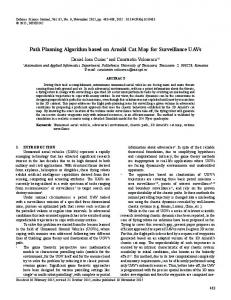
a safe and smooth object path by minimizing the potential function locally for obstacle avoidance, while the gross robot movement is subject to the constraints derived from the topology of the path given a priori. Since the potential is minimized for obstacle avoidance only, its local minima do not cause a problem in the path planning. In this paper, the potential field model in (Chuang, 1998), as reviewed in the next section, is adopted to model the workspace for the path planning of robot manipulators. While the potential model presented in (Chuang, 1998) is readily applicable to path planning for a point robot, a sequential planning algorithm is developed in this paper for manipulators, represented by point samples, of many degrees of freedom (DOFs). The approach computes repulsive force and torque between objects in the workspace. This approach is similar to electrostatics. A collision-free path of a manipulator can then be obtained by locally adjusting the manipulator configuration to search for minimum potential configurations using these forces and torques. The proposed approach uses one or more guide planes (GPs) among obstacles in the free space as final or intermediate goals in the workspace for the end-effector of the manipulator to reach. These GPs provide the manipulator a general direction to move forward and also help to establish certain motion constraints for adjusting manipulator configuration during path planning, as discussed in Section III. Compared to other approaches, the proposed approach is unique in the sense that, under the aforementioned constraints, only the potential function is considered in the derivation of an optimal manipulator configuration (through potential minimization). In Section IV, simulation results are presented for path planning performed for manipulators in different 3-D environments. Section V gives conclusions for this work. II. GENERALIZED POTENTIAL FIELDS IN THE 3-D SPACE In (Chuang, 1998), it is shown that the Newtonian potential, being harmonic in the 3-D space, can not prevent a charged point object from running into another object whose surface is uniformly charged. This is because the value of such a potential function is finite at the continuously charged surface. Subsequently, generalized potential models are proposed to assure collision avoidance between 3-D objects. The generalized potential function is inversely proportional to the distance between two point charges to the power of an integer and, as reviewed next, the potential, and thus, its gradient due to polyhedral surfaces, can be calculated analytically. The path planner proposed in this paper will use these results to evaluate the

n

S u ∆S l

Fig. 1 A polygonal surface S in the 3-D space

repulsion between manipulators and obstacles. Considering a planar surface S in the 3-D space as shown in Fig. 1, the direction of its boundary, ∆S, is determined with respect to its surface normal, n, by the right-hand rule, u × l = n, where u and l are along the (outward) normal and tangential directions of ∆S, respectively. For the generalized potential function, the potential value at point r is defined as {

{

S

{

{

{

dS , m ≥ 2, Rm

{

(1)

where R = |r’ – r| for point r’, r’ ∈ S, and integer m is the order of the potential function. The basic procedure to evaluate the potential at r is similar to that outlined in (Wilton et al., 1984) for the evaluation of the Newtonian potential (m = 1) and can be summarized as follows: (i) Write the integrand of the potential integral over S as surface divergence of some vector function. (ii) Transform the integral into the one over ∆S based on the surface divergence theorem. (iii)Evaluate the integral as the sum of line integrals over edges of ∆S. Related geometric quantities associated with an edge Ci of S in the plane containing S, Q, are shown in Fig. 2 for r’ ∈ C i. Without loss of generality, it is assumed that ∆ d = n . (r – r′) > 0, {

(2)

which is equal to the distance from r to Q. For (i), we have (see (Chuang, 1998)) 1 = ∇ ⋅ ( f (R)P) , S m Rm

(3)

where P is the position vector of r′ with respect to the projection of r on Q, r Q, and

C. C. Lin and J. H. Chuang: A Potential-Based Path Planning Algorithm for Hyper-Redundant Manipulators

O (origin)

Since f m, i(l i) is a rational function for even m’s when m ≠ 2 and is rationalizable for odd m’s (see (Bers and Karal, 1976)), the line integrals can always be evaluated in closed form except for m = 2. For example, if P i0 ≠ 0, we have

r rQ d

r′

R+

n

li +

R–

l+

Ci

R

l–

Geometric quantities associated with a point, an edge C i (subscript i is omitted) of S shown in Fig. 1 and the plane Q containing S

log R , R2 – d 2

fm(R) =

(4)

(m – 2)R m – 2(R 2 – d 2)

. m≠2

Note that if r Q is inside S, f m (R) will become singular for some r′′ = r Q, i.e., R = d. Let S ε denote the intersection of S and a small circular region on Q of radius ε and centered at r Q, the potential due to S can be evaluated as

S

dS = lim Rm ε → 0

=

∆S

S – Sε

∇ s ⋅ ( fm(R)P)dS +

fm(l)P ⋅ udl + lim

ε→0

= Σ Pi0 ⋅ u i i

Ci

α 0

Sε

ε 0

(5)

where

fm, i(l i) = fm(R =

g m(α) =

l i 2 + d 2 + (Pi0) 2 ) ,

α logd ,

(6)

m=2

α , m>2 (m – 2)d m – 2

.

(7)

P i0 is the distance between r Q and C i, l i is measured from the projection of r on C i along the direction of li, and α is the angular extent of the circumference of S ε lying inside S as ε → 0.

1

Φ (x, y, z) = Σ [φ(x2i , y2i , z) – φ(x1i , y1i , z)] + α Z i

φ(x, y, z) = 1z tan – 1

xz , y x2 + y2 + z2

(9)

(10)

where the x i – y i – z coordinate system is determined by the right-hand rule for each edge i of the polygon such that z is measured along the normal direction and x i is measured along edge i of the polygon, respectively. Hence, the repulsive force at point (x, y, z) due to polygon j can be denoted as j j j f j = ( fxj, fyj, fz j) = ( ∂Φ , ∂Φ , ∂Φ ) . ∂x ∂y ∂z

dS Rm

pdpdθ (p 2 + d 2) m/2

fm, i(l i)dl i + g m(α) ,

with R – and R + equal to the distances from r to the two end points of C i , respectively. Thus, the repulsive force exerted on a point charge at (x, y, z) due to polygon j, denoted as 1

can be obtained analytically by evaluating the gradient of the potential function for m = 3 with

m=2 –1

f3, i(l i)dl

li –

l –d l +d = 10 tan – 1 i0 – – tan – 1 i0 + , (8) Pi R Pi R Pi d

C

u

P0

Q

f3, i(l i)dl =

P

P

P0

Fig. 2

l

R

R0

{

417

(11)

For the potential-based path planning of manipulators, the evaluation of the repulsion between manipulators and obstacles involves the calculation of the repulsion between pairs of polygons; each pair has a polygon from the manipulator and the other from obstacles. To simplify the mathematics, links of manipulator are approximately represented by a set of point samples on their surfaces in this paper. Usually, as shown in Fig. 3, the sampling points are located on the vertexes and edges of links and their distribution should be as uniform as possible. Assume that a link has m point samples and the obstacles have n polygon surfaces. If the repulsive force between point sample p k and surface S j is dej noted as f k, the repulsive force exerted on p is equal to n

n

n

j

j

j

fk = (Σ fkjx, Σ fkjy, Σ fkjz)

(12)

according to Eq. (11), and the total repulsive force

Detailed discussions concerning some special cases for the potential calculation, e.g., for P i0 = 0 or d = 0, etc., as well as the associated collision avoidance property can be found in (Chuang, 1998). In this paper, only m = 3 is considered.

418


Fig. 3 The sampling model for a link of a manipulator

GP2

GP2

GP1

(a)

GP1

(b)

Fig. 4 A manipulator is moved toward the goal (not shown) by sequentially traversing a sequence of GPs

exerted on the link can be evaluated as m

f = Σ fk .

(13)

traversal of a given sequence of GPs by the end-effector is regarded as a global solution of the path planning problem for a manipulator.

k

The repulsion expressed by Eq. (13) will be used in the potential-based path planning for robot manipulators in 3-D workspace, as discussed next. The total repulsive torque exerted on a link with respect to a point, say a joint, can be derived similarly. These are omitted for brevity. III. PATH PLANNING The application of the potential model reviewed in the previous section for path planning of manipulators will be discussed in this section. The approach computes repulsive forces and torques experienced by each rigid component, e.g., a link, of a manipulator. A collision-free path of the manipulator can then be obtained by locally adjusting its configuration along the path for minimum potential using these force and torque. In this paper, spherical joints are adopted to connect links of a manipulator since its high DOF can take full advantage of the proposed potential minimization algorithm. For a rough description of a manipulator path, the proposed approach uses one or more guide planes (GPs) as final or intermediate goals in the 3-D workspace. The GPs are polygons among obstacles in the free space, providing the manipulator a general direction to move forward 2 (see Fig. 4). A collision-free 2

1. Generation and Selection of initial GPs In the proposed algorithm, the GPs provide the robot a general direction to move forward. The selection of the initial GPs may be based on (i) their density along the passage, (ii) the visibility between two adjacent GPs, or (iii) the angular variation of two adjacent GPs. For the examples considered in this paper, the initial GPs are selected arbitrarily and the algorithm seems to work reasonably well in terms of the sensitivity of the planned path to the selection of initial GPs. Often, these initial GPs can also be obtained from the Generalized Cylinder (GC) (Nevatia and Binford, 1977) representation as crosssections perpendicular to the GC axis. Fig. 5(a) shows a passage which has approximately rectangular crosssections, and an axis of its GC representation. In general, there is no limit on the number of cross-sections and their shapes are not explicitly specified in advance. In the proposed approach, the shape of the GPs is usually not critical as long as the GPs are confined in the free space. In fact, only the normal direction of a GP, e.g., the direction of the GC axis, is important. Such an axial representation can also be derived from (i) the global navigation function as in (Barraquand and Latombe, 1991; Koditschek, 1987; Yeh and Lu,

The local minimum in potential is not a problem since the proposed algorithm uses GPs as the global planner. The potential function is only used to adjust the configuration of the manipulator to avoid obstacles.


(a)

419

(b)

Fig. 5 The generalized cylinder presentation of a passage

GP1′

GP1 p

GP1′ p′

u

c v

p

p

(a) Fig. 6

GP1′

(b)

(c)

Basic path planning procedure for a given GP (see text). (a) Moving toward the intermediate goal. (b)-(c) two univariant optimization procedures

2003; Lai et al., 2007), as well as (ii) the tree structure representation of free space obtained from the wavefront expansion presented in (Brock and Kavraki, 2001). While the gradient of (i) leads a point object to the goal, global connectivity of free space is available in (ii) and is used in (Brock and Kavraki, 2001) to solve a planning problem in low dimensions. 2. Basic Procedure of Path Planning In this paper, the proposed path planning approach derives a series of minimum potential configurations along the path of a manipulator by locally adjusting its configuration for minimum potential using the results given in Section II. Assuming that a guide plane GP 1 is given as an intermediate goal, the basic path planning procedures for moving the end-effector p′ of a manipulator onto GP 1 include (see Fig. 6): (i) Translate the distal links of the manipulator to move its end-effector p′ toward the GP 1 . If p′ can not reach GP 1 directly, e.g., due to collision, a virtual intermediate plane GP′1 is inserted as shown in Fig. 6(a). In this step, an intermediate

simple solution of the inverse kinematics problem is obtained by translating all manipulator links except for the two base links, the base link and the link connected to it. For each translation, the two base links, together, can have at most three DOFs. (ii) Search for the minimum potential configuration of the manipulator for p ∈ GP′1 by repeatedly executing: (a) Search for the minimum potential configuration of the manipulator with the distal link fixed in orientation. The minimization is performed by sliding p along two orthogonal di→ → rections on GP′1, e.g., u and v. (Fig. 6(b)) (b) Search for the minimum potential configuration of the manipulator with the endeffector p fixed in position. The minimization is performed by changing the orientation of the distal link with p as its rotation center. (Fig. 6(c)) In this step, the problem is solved by finding a sequence of sub-optimal solutions with monotonically decreasing potential. Finally, the minimal potential solution is found in (iii). (iii) Repeat (i) and (ii) until p reaches GP 1.

420


In general, there are different ways to change the manipulator configuration to move p toward GP 1. A simple translation of distal links is adopted in (i) as a preliminary implementation of our algorithm. As shown in Fig. 6(a), the translation of the distal links is carried out to move the end-effector from p′ to c, where c is the centroid of GP 1. If collision occurs or if the connectivity of manipulator can not be maintained, the distance of the translation is reduced until the translation is collision-free while the manipulator remains connected. Accordingly, a new GP is inserted, e.g., GP′1 . No configuration improvement to reduce the repulsive potential is considered at this stage. As for the search for the minimum potential configuration of the manipulator in (ii), links of the manipulator are adjusted from the distal link to the base link using the repulsion experienced by the manipulator. The distal link has five DOFs, i.e., two for its location for p ∈ GP′1 and three for its orientation. While each of other distal links has three DOFs for its orientation, the two base links, together, have at most three DOFs with their connecting joint being constrained to lie on a circle. In (ii), the associated constrained optimization problem is divided into two iterative univariant optimization procedures (Beveridge and Schechter, 1970), as in (ii-a) and (ii-b). In (ii-a), the distal link is fixed in its orientation (see Fig. 6(b)) as p slides on GP′1 to search for the minimal potential configuration and other distal links are sequentially adjusted in orientation, staring from the link connected to the distal link. In (ii-b), the distal link is adjusted in orientation while fixed in position (see Fig. 6(c)) and the procedure for adjusting the rest of the links is similar to that in (iia). For a particular GP, say GP′1 in Fig. 6, (ii-a) and (ii-b) are repeatedly performed until negligible changes in the manipulator configuration are obtained. Then, another intermediate GP which is closer to GP 1 is obtained with (i) and the process repeats. The path planning algorithm, as summarized below, ends as the end-effector reaches the given GP1 or an infeasible problem. Detailed implementation of the algorithm is presented in the next subsection. Algorithm End_Effector_to_GP Step 0 Initialize δ = p′c and GP ← GP 1. Step 1 Translate the distal links of the manipulator with distance δ to move p′ to p along the direction of p′c . Find the smallest n ≥0 such that δ ← δ / 2n corresponds to a feasible and collision-free translation. If δ < δmin, go to Step 6; otherwise, construct GP′1 with GP′1 || GP1 and p ∈ GP′1, and let GP ← GP′1. (see Fig. 6(a)) Step 2 Translate the distal link by sliding p on GP to minimize the potential. (see Fig. 6(b))

Step 3 Adjust joint angle of the manipulator for the minimum potential configuration with p fixed in position. (see Fig. 6(c)) Step 4 Go to Step 2 if the translation in Step 2 or the joint angle adjustment in Step 3 is not negligible. Step 5 If p reaches GP1, the planning is completed. Otherwise, p′ ← p and go to Step 1 with δ = p′c. Step 6 Exit and report that GP 1 is unreachable. For path planning involving multiple GPs, the above algorithm will be executed for each of them sequentially. It is assumed that the planning for a GP starts as the planning of the previous GP is accomplished. The path planning ends as the end-effector reaches the goal, which is usually a (goal) GP in the path planning problems considered in this paper. 3. Implementation Details 1) Step 1 of Algorithm End_effector_to_GP: In Step 1 of End_effector_to_GP, as mentioned earlier, the translation of distal links is achieved in the implementation by translating every link except the two base links. The configuration of the two base links is determined simply by considering a planar motion on the plane formed by J 0 (the base joint), the old position of J 1 and J 2 such that an additional rotation will move J2 to its new location. On the other hand, there are different ways to move p′ toward GP 1 . For example, p′ can be moved toward GP 1 in the direction perpendicular to GP 1 . In our simulation, for simplicity, the end-effector is translated from p′ to p by distance δ = max(p′c/2 n); n ≥ 0, along the direction of p′c . If GP 1 is directly reachable without any collision and disconnection of the manipulator, p and c are identical. A threshold, i.e., δ min = 1% of workspace size, is established to set a lower bound of the magnitude of allowed translation. A translation which requires a smaller movement, δ < δ min , indicates an infeasible path planning problem. While no configuration improvement to reduce the repulsive potential is considered in the above translation procedure, Steps 2 and 3 minimize the potential through constrained optimization procedures. To that end, an intermediate GP, GP′1, is added along the path to serve as a geometric constraint for successive adjustments of manipulator configuration. Again, as long as p ∈ GP′1, the choice of the orientation of GP′1 is not unique. For simplicity, GP′1 || GP 1 is adopted in our simulation. 2) Adjusting end-effector position in Step 2: After the end-effector reaches p, as shown in Fig. 6(b), one of the univariant procedures, which allows the distal link to adjust its location, but not its

421


orientation, in minimizing the repulsive potential, is performed in Step 2 of End_effector_to_GP. Since the minimization is constrained by p ∈ GP, only the projection of the resultant force experienced by the distal link on GP is taken into account. Consider the forces exerted on the distal link lnk n, as shown in more detail in Fig. 7. Let f 1 be the repulsive force exerted on lnk n due to the repulsion between lnk n and the obstacles, and f 2 be the force exerted on J n – 1 due to the repulsive torque, denoted as τ 0, between other manipulator links (lnk 1 through lnkn – 1) and obstacles. For a univariant minimization approach, only one variable is adjusted at a time. To determine the minimum potential location of lnk n as p sliding on GP, all of the joint angles of the manipulator, except the base joint J 0, are assumed to be fixed. Therefore, τ 0 can be calculated by considering a single rigid composite link formed by lnk 1 through lnk n – 1 with respect to J 0. Thus, f2 =

τ0 , l0

(14)

where l 0 is the length of J 0J n – 1 . To determine the direction in which p should slide on GP, and thus lnkn should translate, to reduce the repulsive potential, the projection of the result→ ant force exerted on lnk n along an arbitrary u || GP f u = f 1u + f 2u

(15)

is calculated, where subscript u denotes the projec→ tion along u. To move link n such that the potential → will have maximum rate of reduction, u can be cho→ → sen as the projection of f1 + f2 on GP. A gradientbased binary search for the minimum potential location of → p along u can then be performed using (11). The initial step of sliding is arbitrarily chosen as 10% of the → workspace size. If the movement of lnk n along u or f u is negligible, e.g., the movement is smaller than 1% of workspace size, another minimizing scheme → → along v ∈ GP, which is orthogonal to u, is performed to minimize f v . Step 2 ends when two consecutive binary searches along the two orthogonal directions result in negligible movement of lnk n. In the above search processes, each time the position of p is changed, the orientation of rest links, i.e., joint angles at J 0 through J n –1 , need to be adjusted for connectivity and for minimum potential of the manipulator. Such a procedure is very similar to the joint angle adjustment performed in Step 3 of End_effector_to_GP, as discussed next. 3) Adjusting joint angle in Step 3: Once the minimum potential position of lnkn is determined with Step 2 of End_effector_to_GP, another univariant procedure, which allows the distal link to adjust its orientation with end-effector p fixed in position is performed to

GP

u fu

Base Joint J0

v P

f1 lnkn Jn – 1 f2

Fig. 7

Sliding p on GP 1′, by translating lnk n to reduce the repulsive potential

reduce the potential further, as shown in Fig. 6(c). Under such a constraint, the distal link can rotate with respect to p to reduce the repulsive potential. The direction in which the distal link should rotate is determined by the repulsive torque experienced by the distal link with respect to p. Let τ n be the repulsive torque experienced by lnk n with respect to p due to the repulsion between lnk n and let f 2, as described in the previous subsection, be the force exerted on J n –1 due to the repulsive torque between other manipulator links and obstacles. The resultant torque experienced by lnk n with respect to p is equal to

τ n* = τ n + f 2⊥ . l n,

(16)

where ln is the length of lnk n and f2⊥ is the projection of f 2 onto a plane perpendicular to lnk n. To find the minimum potential orientation of lnk n for p fixed in position, gradient-based binary searches are performed using the projection of τ n * along three orthogonal axes of rotation, one axis at a time. For each binary search, the initial rotating angle is arbitrarily chosen as 5°, while the accuracy in identifying the 1-D potential is chosen as 0.5°. Each time the orientation of lnk n is changed, the orientation of the rest links are adjusted recursively for connectivity and for minimum potential using τ n –1 *, τ n –2 * .... , etc. Step 3 ends if a binary search using τn* results in a negligible change in the orientation of lnk n , i.e., 0.5°. As for the computation complexity, if every link needs k binary searches on the average to find the best orientation, the total number of binary searches needed for the derivation of the minimum potential configuration of an n-link manipulator is equal to k 1 + k2 + ... + kn – 2 = (k n – 1 – k)/(k –1)

(17)

which appears to have a fairly large value. Fortunately, much lower computation complexity is often observed, as in the examples considered in the next section.

422


GP2

GP3

GP1

Fig. 8

(a)

(b)

(c)

(d)

(e)

(f)

(g)

(h)

(i)

(j)

A path planning example for a 6-link manipulator in a 3-GP workspace. (a) The three predetermined GPs. (b)-(j) Side views of intermediate configurations of the manipulator which grabs an object at GP2 and transports it to GP 3

GP4 GP3 GP2 GP1

(a)

(d)

Fig. 9

(b)

(e)

(f)

(c)

(g)

(h)

A path planning example for a 6-link manipulator in a 4-GP workspace. (a) The initial configuration. (b)-(c) Two different views of the final configuration. (d)-(h) Top views of the initial configuration of the manipulator, as well as intermediate configurations as its end-effector reaches each of the four GPs

IV. SIMULATION RESULTS In this section, simulation results are presented for path planning performed on a Windows system for manipulators in a 3D environment. Fig. 8(a) shows the three GPs predetermined through global path planning. Side views of intermediate configurations of the manipulator are shown as it grabs an object at GP2 (Figs. 8(b)-(d)) and transports it to GP3 (Figs. 8(e)-(j)). The simulation takes a total of 3.624 seconds to plan a 10-configuration collision-free path. Due to the repulsion of the cubic obstacle on the top of the passage, the manipulator detours around the

obstacle with its links basically lying in the middle of the workspace. It is readily observable that these trajectories are safe and smooth. Figures 9(a)-(c) show the initial and final configurations of the path planning for another 6-link manipulator stretching into a tapered passage with 4 GPs. The passage makes up, down and right turns at GP 1, GP 2 and GP 3, respectively. Fig. 9(a) shows the initial configuration of the manipulator which lies in a plane parallel to GP 1. Figs. 9(b)-(c) show top and side views, respectively, of the final configuration indicating that the end-effector of the manipulator reaches the final GP safely. Figs. 9(d)-(h) show the


423

Table 1 Computation time for manipulator configurations shown in Fig. 10 Computation times (sec) config. config. config. config. config. config.

1: 2: 3: 4: 5: 6:

5.988 3.245 1.612 2.184 1.592 1.492

config. config. config. config. config. config.

7: 1.963 8: 1.612 9: 1.472 10: 1.502 11: 2.374 12: 1.612

Total time: 26.648

(a)

(b)

(d)

(c)

(e)

Fig. 10 (a) The complete manipulator trajectory. (b) The partial trajectory between Figs. 9(d) and (e). (c) The partial trajectory between Figs. 9(e) and (f). (d) The partial trajectory between Figs. 9(f) and (g). (e) The partial trajectory between Figs 9(g) and (h)

top views of the initial configuration of the manipulator, as well as intermediate configurations as its end-effector reaches each of the four GPs. Figures 10(a)-(e) show complete as well as partial manipulator trajectories. In order to show the manipulator trajectory more clearly, configurations obtained by End_Effector_to_GP are shown in different gray levels, i.e., the initial configuration is shown in white while final configuration is shown in black. The planned manipulator path is also observed to be safe and smooth. The simulation takes a total of 26.648 seconds to plan the 12-configuration collision-free path and the computation time for each configuration is shown in Table 1. While the differences in the amount of CPU time required to compute different manipulator configurations are mostly insignificant, it takes much more time to compute the first configuration. This is because the first configuration, which can be seen clearly in Fig. 10(b), requires the most adjustments in manipulator joint angles from the previous (initial) configuration. Figures 11(a)-(c) show the initial (from two different views) and final configurations, respectively, of the path obtained for a 6-link manipulator working in a blocked workspace. Figs. 11(d)-(f) show side views of the intermediate configurations as its end-effector reaches each of the three GPs. Figs. 11(g)-(i) show top views of the same manipulator configurations. It can be seen clearly from Figs. 11(d)(i) that the end-effector of the manipulator reaches

the three GPs safely. Figures 12 show side views and top views, respectively, of some partial trajectories of the manipulator. The safety and smoothness of the manipulator trajectory is also observed. The simulation takes a total of 34.199 seconds to plan a 11-configuration collision-free path. Because the workspace is more complex, the path planning is more time-consuming than other examples. V. EXTEND TO DUAL-ARM SYSTEM While only one robot in a workspace limits the classes of tasks that can be performed, a multi-robot system can expand the application area of robots. For example, a dual-manipulator system is more efficient than a single-manipulator system since the tasks can be processed in parallel. In this section, the proposed algorithm is extended to a dual-arm system. The proposed method uses a master-slave scheme to deal with the coordination of two manipulators, by alternately identifying the two manipulators as a master robot and a slave robot, respectively. The alternate priority algorithm has two stages. In the first stage, the master manipulator adjusts its configuration by using the repulsion between the master manipulator and obstacles, including the slave manipulator. Once the adjustment of the master is done, the slave begins to move toward its intermediate goal and adjusts its configuration by using the repulsion between the slave and obstacles, including the master. These two stages are processed

424


GP3

GP1

GP3

GP1 GP2

GP2

(a)

(b)

(c)

(d)

(e)

(f)

(g)

(h)

(i)

Fig. 11 A path planning example for a 6-link manipulator in a 3-GP blocked workspace. (a)-(b) Two different views of the initial configuration. (c) The final configuration. (d)-(f) Side views of the intermediate configurations as its end-effector reaches each of the three GPs. (g)-(i) Manipulator configurations observed from a different viewing angle

iteratively until both manipulators reach their goals. Considering two manipulators trying to position their end-effectors to their goals while avoiding obstacles (including another manipulator), as shown in Fig. 13. The two manipulators are specified as the master manipulator and the slave manipulator, respectively. Fig. 14 shows the planned trajectories of a dual-arm system. The initial configuration of this example is shown in Fig. 14(a). The proposed algorithm plans a nine-configuration path for the master and a seventeenconfiguration path for the slave. The total computation time is 6.547 seconds (0.235s for the master and 6.312s for the slave). VI. CONCLUSIONS In this paper, a potential-based algorithm for a robot manipulator is proposed to solve path planning

problems in variant 3-D workspace. The proposed algorithm uses an artificial potential field to model the workspace wherein obstacles’ surfaces are assumed to be charged uniformly and the manipulator is represented as a set of charged sampling points. The repulsive force and torque between manipulator and obstacles thus modeled are analytically tractable, which makes the algorithm efficient. To give a general path direction, a sequence of GPs to be reached by the manipulator are assumed to be given in advance in the workspace. As a GP is an intermediate or final goal for the end-effector of a manipulator to reach, it also helps to establish certain motion constraints for adjusting manipulator configuration during path planning. According to such constraints, the proposed approach derives the path for a manipulator by adjusting its configurations at different locations along the path to minimize the potential using the above


(a)

(b)

(c)

(d)

(e)

(f)

425

Fig. 12 (a) The partial trajectory between Figs. 11(a) and (d). (b) The partial trajectory between Figs. 11(d) and (e). (c) The partial trajectory between Figs. 11(e) and (f). (d)-(f) Manipulator trajectories observed from a different viewing angle. It is easy to see that the manipulator does not collide with obstacles from these figures. For example, the distal link seems to collide with a face of the obstacle in (a) and (b), but, as one can see in (d)-(e), it is collision-free. In (c), two distal links seem to collide with another face, but (f) shows that the two distal links do not collide with that face

Goal of Slave

Slave

in this paper, the proposed approach can be extended to a workspace with moving obstacles with essentially no change in the path planning algorithm. ACKNOWLEDGMENTS

Master

Goal of Master

Fig. 13 A dual-manipulator system has two 7-link manipulators, Master and Slave, their goals

forces and torques. Simulations show that a path thus derived is always spatially smooth and effective. Since the proposed approach uses workspace information directly, it is readily applicable to hyper-redundant manipulators. Furthermore, the proposed algorithm can be extended to multi-arm systems. An example of a dual-arm system is also given in this paper. In the proposed algorithm, the master robot plans a local path to its intermediate goal using the repulsion from obstacles and the slave robot firstly. Then, the slave plans its local path using the repulsion from obstacles and the master. The paths can be obtained by executing these two stages iteratively until both manipulators reach their goals. While only static environments are considered

The authors would like to acknowledge the valuable suggestions of reviewers. This work is supported by National Science Council of Taiwan under grant no. NSC 97-2221-E-366-004 and NSC 98-2220-E224-009. NOMENCLATURE f fj j

fk fk m P P i0 S Sε

total repulsive force exerted on a link repulsive force at point (x, y, z) due to polygon j repulsive force between a point sample p k and a obstacle surface S j repulsive force exerted on a point sample pk order of the potential function position vector of r′ with respect to the projection of r on Q distance between r Q and C i planar surface of obstacles in the 3-D space intersection of S and a small circular region

426


(a)

(b)

(c)

(d)

(e)

(f)

(g)

(h)

(i)

( j)

(k)

(l)

(m)

(n)

(o)

(p)

(q)

Fig. 14 The intermediate configurations of the dual-manipulator system in Fig. 13. The master robot plans a local path to its intermediate goal using the repulsion from obstacles and the slave robot firstly. Then, the slave plans its local path using the repulsion from obstacles and the master. The paths are obtained by executing these two stages iteratively

on Q of radius ε ∆S boundary of a planar surface φ (x, y, z) gradient of the potential function Φ (x, y, z) repulsive force exerted on a point charge at (x, y, z) due to polygon j

REFERENCES Barraquand, J., and Latombe, J., 1991, “Robot Motion Planning: A Distributed Representation Approach,” International Journal of Robotics


Research, Vol. 10, No. 6, pp. 628-649. Bers, L., and Karal, F., 1976, Calculus. Holt and Rinehart and Winston, NY, USA. Beveridge, G., and Schechter, R., 1970, Optimization: Theory and application. McGraw-Hill, NY, USA. Brock, O., and Kavraki, L., 2001, “Decomposition-based Motion Planning: A Framework for Real-Time Motion Planning in High-Dimensional Configuration Spaces,” IEEE International Conference of Robotics and Automation, Seoul, Korea, pp. 1469-1474. Brooks, R., and Lozano-Preez, T., 1985, “A Subdivision Algorithm in Configuration Space for Findpath with Rotation,” IEEE Transation on Systems, Man and Cybernetics, Vol. 15, No. 2, pp. 224-233. Chuang, J.-H., 1998, “Potential-Based Modeling of Three-Dimensional Workspace of the Obstacle avoidance,” IEEE Transation on Robotics and Automation, Vol. 14, No. 5, pp. 778-785. Chuang, J.-H., and Ahuja, N., 1998, “An Analytically Tractable Potential Field Model of Free Space and its Application in Obstacle Avoidance,” IEEE Transation on Systems, Man and Cybernetics, Part B: Cybernetics, Vol. 28, No. 5, pp. 729-736. Chuang, J.-H., Tsai, C.-H., Tsai, W.-H., and Yang, C.Y., 2000, “Potential-Based Modeling of 2-D Regions Using Nonuniform Source Distribution,” IEEE Transation on Systems, Man and Cybernetics, Part A: Systems and Humans, Vol. 3, No. 2, pp. 197-202. Conkur, E. S., 2009, “Path Planning Using Potential Field for Highly Redundant Manipulators,” Robotics and Autonomous System, Vol. 57, No. 2, pp. 194-201. Dasgupta, B., Gupta, A., and Singla, E., 2009, “A Variational Approach to Path Planning for Hyperredundant Manipulators,” Robotics and Autonomous Systems, Vol. 57, No. 2, pp. 194-201. Geraerts, R., and Overmars, M. H., 2007, “Reachability-Based Analysis for Probabilistic Roadmap Planners,” Robotics and Autonomous Systems, Vol. 55, No. 11, pp. 824-836. Hwang, Y. K., and Ahuja, N., 1992, “Gross Motion Planning a Survey,” ACM Computing Surveys, Vol. 24, No. 3, pp. 219-291. Kavraki, L. E., Svestka, P., Latombe, J. C., and Overmars, M. H., 1996, Aug.. “Probabilistic Roadmaps for Path Planning in High-Dimensional Configuration Spaces.” IEEE Transation on Robotics and Automation, Vol. 12, No. 4, pp. 566-580. Khosla, P., and Volpe, R., 1988, “Superquadric Artificial Potentials for Obstacle Avoidance and Approach,” IEEE International Conference on Robotics and Automation, pp. 1778-1784. Koditschek, D., 1987, “Exact Robot Navigation by Means of Potential Functions: Some Topological Considerations,” IEEE International Conference of Robotics and Automation, Raleigh, North

427

Carolina, USA, pp. 1-6. Lai, L.-C., Wu, C.-J., and Shiue, Y.-L., 2007, “A Potential Field Method for Robot Motion Planning in Unknown Environments,” Journal of the Chinese Institute of Engineers, Vol. 30, No. 3, pp. 369-377. Latombe, J. C., 1991, Robot Motion Planning. MA: Kluwer, Boston. Latombe, J. C., 1999, “Motion Planning: A Journey of Robots, Molecules, Digital Actors, and Other Artifacts,” International Journal of Robotics Research, Vol. 18, No. 11, pp. 1119-1128. Lin, C.-L., Lin, J.-R., and Jan, H.-Y., 2007, “Singularity Analysis and Path Planning for a Mdof Manipulator,” Journal of the Chinese Institute of Engineers, Vol. 30, No. 5, pp. 917-922. Lozano-Perez, T., 1983, “Spatial Planning: a Configuration Space Approach,” IEEE Transation on Computers, Vol. C-32, No. 2, pp. 108-120. Nevatia, R., and Binford, T., 1977, “Description and Recognition of Curved Objects,” Artificial Intelligence, Vol. 8, No. 1, pp. 77-98. Thanailakis, A., Tzionas, P. G., and Tsalides, P. G., 1997, “Collision-Free Path Planning for a Diamond-Shaped Robot Using Two-Dimensional Cellular Automata,” IEEE Transation on Robotics and Automation, Vol. 13, pp. 237-250. Tsai, C.-H., Lee, J.-S., and Chuang, J.-H., 2001, “Path Planning of 3-D Objects Using a New Workspace Model,” IEEE Transation on Systems, Man and Cybernetics, Part B: Cybernetics, Vol. 31, No. 3, pp. 405-410. Tsourveloudis, N. C., Valavanis, K. P., and Herbert, T., 2001, “Autonomous Vehicle Navigation Utilizing Electrostatic Potential Fields and Fuzzy logic.” IEEE Transation on Robotics and Automation, Vol. 17, No. 4, pp. 490-497. Valavanis, K. P., Herbert, T., and Tsourveloudis, N. C., 2001, “Mobile Robot Navigation in 2-D Dynamic Environments Using Electrostatic Potential Fields,” IEEE Transation on Systems, Man and Cybernetics, Part A: Systems and Humans, Vol. 30, No. 2, pp. 187-196. Wilton, D. R., S. M. Rao, A. W. G., Schaubert, D. H., Al-Bundak, O. M., and Butler, C. M., 1984, “Potential Integrals for Uniform and Linear Source Distributions on Polygonal and Polyhedral Domains,” IEEE Transation Antennas and Propagation, Vol. AP-32, No. 3, pp. 276-281. Yeh, M.-F., and Lu, H.-C., 2003, ”Car-Like Robot Motion Planning Based on Grey Relational Pattern Analysis,” Journal of the Chinese Institute of Engineers, Vol. 26, No. 1, pp. 1–12. Manuscript Received: Dec. 11, 2009 Revision Received: Mar. 17, 2010 and Accepted: Mar. 22, 2010