A Kernel-based Approach to Document Retrieval Albert Gordo
Jaume Gibert
Ernest Valveny
Computer Vision Center Dept. of Computer Science Campus UAB, Ed. O, 08193 Bellaterra (Barcelona), Spain
Computer Vision Center Dept. of Computer Science Campus UAB, Ed. O, 08193 Bellaterra (Barcelona), Spain
Computer Vision Center Dept. of Computer Science Campus UAB, Ed. O, 08193 Bellaterra (Barcelona), Spain
[email protected]
[email protected] Marçal Rusiñol
[email protected]
Computer Vision Center Dept. of Computer Science Campus UAB, Ed. O, 08193 Bellaterra (Barcelona), Spain
[email protected] ABSTRACT In this paper we tackle the problem of document image retrieval by combining a similarity measure between documents and the probability that a given document belongs to a certain class. The membership probability to a specific class is computed using Support Vector Machines in conjunction with similarity measure based kernel applied to structural document representations. In the presented experiments, we use different document representations, both visual and structural, and we apply them to a database of historical documents. We show how our method based on similarity kernels outperforms the usual distance-based retrieval.
Categories and Subject Descriptors I.7.5 [Document and Text Processing]: Document Capture—Document analysis; H.3.7 [Information Storage and Retrieval]: Digital Libraries
General Terms Algorithms
at the image level, with respect to a reference one, i.e., a query-byexample document image retrieval. This is usually accomplished establishing a distance or similarity measure between documents in the collection and the query and sorting them accordingly. However this approach presents some caveats. When retrieving similar documents, it is usually expected that such documents also belong to the same category than the query one. For example, when retrieving letters, we are interested in obtaining similar documents that are also letters. If we perform an ordering solely based on the similarity measure, it is likely that similar documents belonging to different classes will score better than slightly different documents from the same class. This is particularly true when documents contain a high inter-class variability. For this reason, it seems important to take into account the likelihood that documents belong to the same class when performing the retrieval. To do so, we will make use of Support Vector Machines (SVMs) that allow us to obtain the probabilities of such document belonging to any of the classes. Using this information, documents can be ordered and retrieved by the probability of belonging to the same class.
Keywords Document retrieval, Support Vector Machines, Similarity measure based kernels, query-by-example
1. INTRODUCTION Digital libraries usually contain huge amounts of heterogenous documents. When we consider typewritten documents, OCRs are used to transcribe them in order to provide access to the text. However, there are many cases where an OCR can not be used, as for instance handwritten or graphic-rich documents, hindering the accessibility to these collections. In this particular scenario, it is interesting to propose methodologies that aim to retrieve documents by similarity
Permission to make digital or hard copies of all or part of this work for personal or classroom use is granted without fee provided that copies are not made or distributed for profit or commercial advantage and that copies bear this notice and the full citation on the first page. To copy otherwise, to republish, to post on servers or to redistribute to lists, requires prior specific permission and/or a fee. DAS ’10, June 9-11, 2010, Boston, MA, USA Copyright 2010 ACM 978-1-60558-773-8/10/06 ...$10.00
The main contribution of this work is the comparison between both query-by-example ways of retrieving documents. The first one just uses a similarity measure between documents to check their proximity to a query document. The second one makes use of SVMs to compute the probability of each document of belonging to every specific document class and then sort documents not by proximity but by probability of belonging to the same class. In this way, documents that are unlikely to belong to the same category will not rank high even if their distance is low. In the same way, documents that have a high probability of belonging to the same class will have a higher rank, even if the distance between them is high. In order to test both procedures in different scenarios, we have used three different document representations, namely, a vectorbased representation which makes use of a densities decomposition [9] and two structural representations, the Minimum Weight Edge Cover (MWEC) [10] and the Polar Graph representation [7], along with their associated distances. Classification of structural representations of documents via SVMs is not straightforward. To overcome this problem, kernels for struc-
tured data can be used. Then, to make the comparison as fair as possible and to relate both ways of retrieving documents, we have considered several kernels for structured data which directly depend on a similarity measure between documents. We finally show how this way of tackling with document retrieval outperforms the usual distance-based one. The rest of the paper is organized as follows. Section 2 is devoted to formalize which is the protocol we use for retrieving documents after a probability of belonging to each class is computed for all documents. Such computation is done using SVMs in conjunction with similarity-based kernels which are introduced and summarized in Section 3. Following we describe, in the experiments section, the database we have used, the document representations we have chosen, the training and testing protocols and the obtained results. Finally, in Section 5, the conclusions of the work are outlined.
2. DOCUMENT RETRIEVAL The Document Image Retrieval problem has been reviewed by Doermann in [4], by Mitra and Chadhuri in [13] and by Marinai in [12]. These authors identified two different retrieval paradigms, namely, the recognition-based retrieval and the similarity-based retrieval schemes. In the first case, document image analysis techniques are used to extract the documents’ contents. These contents can be of textual nature (by the use of an OCR) or can be semantic meta-data (e.g. keywords, predefined document categories, etc.). In these systems the query formulation is done at textual or symbolic level. The major drawback of this paradigm is that the retrieval performance relies on the recognition ability which in some documents (e.g. historical or handwritten documents) might be low. On the other hand, we have the similarity-based retrieval systems which expect a document image to act as query. They try to retrieve similar documents to the query image without explicitly recognizing the documents’ contents nor manually annotating the documents with predefined meta-data. Such query formulation can be referred as query-byexample. These methods, however, completely ignore the notion of document categories which in some cases might be very useful. We propose in this paper a combination of both strategies, i.e. a query-by-example system which also uses a document categorization. By these means we allow a retrieval based on the probability that the query document belongs to a certain class. Given a query document q, we want to retrieve the documents in the dataset sorted with respect to this query. Typically such sorting is made by the proximity of the elements to the query object. For such task, some document distance must be defined, and this distance will depend on the document representation. For instance, in the case of graph-based representations, the graph edit distance could be a suitable choice. For fixed length representations, e.g. based on a densities decomposition [9] or the run-length histograms [11], histogram distances as χ2 could be used. We tackle this task in a different way. Instead of a proximity criterion we take the probability of two documents of belonging to the same class. Specifically, we proceed in the following way. Using kernel machines (particularly, SVMs), every document can be represented (after training and classification) as a vector of probabilities, where each entry refers to the probability of belonging to a certain class. Formally, given a set of classes C = {c1 , c2 , . . . , cN } and a document d, the output of classification is a vector d ∼ ( d1 , d2 , . . . , dN ),
(1)
where di is the probability of∑the document d to belong to class ci , di = P (d ∈ ci ), and where N i=1 di = 1. After this step, we rank all the documents with respect to the query document q by computing, for each document t, the probability of belonging to the same class, this is, by calculating P (C(q) = C(t)). Given a document t, the probability that q and t belong to the same class is P (C(q) = C(t)) = P (q, t ∈ c1 ) ∪ · · · ∪ P (q, t ∈ cN ) =
N ∑
P (q, t ∈ ci ) =
i=1
=
N ∑
N ∑
P (q ∈ ci ) ∩ P (t ∈ ci )
i=1
qi · ti = ⟨q, t⟩,
(2)
i=1
where ⟨·, ·⟩ denotes the standard inner product. Note that the inner product over normalized vectors corresponds to the cosine of the angle between such vectors, which has already been used as a similarity measure in different contexts. Training and classification of documents with fixed-length representations using Kernel Machines is straightforward. However, their use over structured data as graphs is not trivial, and kernels for structured data must be used. Section 3 describes some known basic kernels for this kind of structures and how they will be used in our approach.
3.
BACKGROUND ON KERNELS
In this paper we adopt a kernel-based approach for document retrieval. This section is devoted to summarize the main concepts related to kernel machines and the kernels we have used.
3.1
The kernel trick
Kernel machines are a wide set of machine learning techniques that have been lately gaining a lot of popularity. Their main advantage over other techniques is that they do not necessarily need a vectorial representation of data but other kind of representations, such as strings or graphs, are also supported. Kernel machines work by defining a similarity measure between pairs of patterns to be processed; this measure is a kernel function. On the other hand, every data analysis method that depends only on inner products between pairs of objects can be easily converted into a kernel machine by changing the inner product for a kernel function: such procedure is called the kernel trick. This fact holds in a theorem which claims that every kernel can be understood as an inner product in an implicit Euclidean space where data is embedded. In a formal way, given a kernel function k : X × X → R, there always exists a map ψ : X → H such that k(x, y) = ⟨ψ(x), ψ(y)⟩.
(3)
Here by, X is the space of objects or patterns under study and H is an unknown -in the sense of implicit- inner product space. Support Vector Machines are a good representative of kernel machine where the kernel trick plays an important role. Provided a positive definite kernel, SVMs separate classes of patterns by maximizing margins using optimal hyperplanes in the implicit Euclidean space of the kernel [15].
3.2
Kernels based on similarity measures
In this paper, we are essentially working with similarity measures between document layouts. As we just said, kernel machines -and SVMs in particular- need to define a similarity measure between documents, a kernel function. Also, as we already said, we want to compare both ways of retrieving documents, namely, a distancebased and a kernel-based. This immediately suggests the use of kernels that depend on similarity measures. Some examples of these kind of kernels are described in [14] where kernels between graphbased representations are defined using graph edit distance as the similarity measure. We have used some of these kernels in our work, which we will now summarize. Given d(x, y) a similarity measure between two documents, in which similar documents will have low similarity or distance values and dissimilar documents will have high values, we consider the functions k1 (x, y) = −d(x, y)
(4)
k2 (x, y) = −d(x, y)
(5)
k3 (x, y) = exp(−d(x, y))
(6)
2
k4 (x, y) = tanh(−d(x, y)).
(7)
These functions try to follow the idea of giving high kernel values when objects are similar and low kernel values when they are dissimilar. This can be seen as a generalization of the inner product in an Euclidean space, where vectors pointing in the same direction have high inner product values and vectors pointing in opposite directions have low inner product values. We have also considered, in a similar way as it is done in [1], an adaptation of the common Gaussian kernel for vectorial data. This is done by replacing the Euclidean distance of the vectors by the similarity measure of the objects we consider. It leads to the following kernel ( ) 1 k5 (x, y) = exp − 2 d(x, y)2 . (8) 2σ
3.3 Discussion and a reference kernel The kernel functions described in the previous section are, in general, non-positive definite. This fact does not fit in the mathematical foundations of the SVMs technique in which the kernel functions need to fulfil certain properties, such as positive definiteness and symmetry. In that case, kernels are called valid kernels. However, there are theoretical evidences showing that SVMs learning in conjunction with non-positive definite kernels may have a clear interpretation of hyperplane classifiers, not by margin maximization in Euclidean spaces, but by minimization of distances between convex hulls in pseudo-Euclidean spaces [8]. It is also worth noticing that the use of such functions often leads to good results as shown in [3], which agrees with our results as it will be shown later. Nevertheless, for the sake of completeness of the work and due to the fact that our retrieval approach is taken from a kernel point of view, we have also used a valid kernel in our experiments. This kernel also depends on the similarity measure between the documents but in a rather different manner. The kernel is obtained after explicit embedding of the documents in a vector space. Then, the kernel is computed as the regular inner product in this vector space. The embedding is performed based on the distance of the documents to a given set of prototypes [2], as described in the following. Formally, let {pi }n i=1 ⊆ X be a set of object prototypes or repre-
sentatives. Given an object x ∈ X the embedding of x in a vector space is defined by ϕ : X → Rn x 7→ ϕ(x) = (d(x, p1 ), . . . , d(x, pn )).
(9)
Using embedding (9) we just consider the inner product in the new vector space, leading to the last kernel we have taken into account: k6 (x, y) = ⟨ϕ(x), ϕ(y)⟩.
4.
(10)
EXPERIMENTS
In this section we will describe the experiments performed to compare both query-by-example retrieval methods, ordering by distance and ordering by same class probability. Subsections 4.1 and 4.2 deal with the dataset we will be using and the different document representations we have used. Subsection 4.3 explains the experimental setup and training and testing protocols, and finally Subsection 4.4 presents the obtained results.
4.1
Dataset
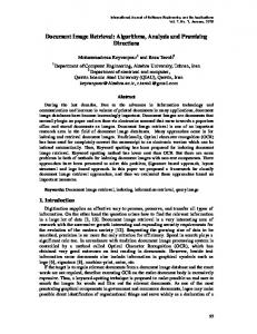
To evaluate these retrieval methods we will test them against the Girona Archives database. The Girona database is a collection of documents from the Civil Government of Girona, in Spain, that contains documents related to people going through the SpanishFrench border from 1940 up to 1976 such as safe-conducts, arrest reports, documents of prisoners transfers, medical reports, correspondence, etc. Even if it is a mostly-text database, in this case most of the pages also have images like stamps, signatures, etc, in a non-manhattan disposition. We have used a subset of the database which contains 743 images and is currently divided in 8 different categories. Some of these images are slightly skewed, but in most cases the skew is almost non-existent. Some samples of the database can be seen in Figure 1.
4.2
Document representations
For this task, we will use two structural representations based on the layout of the documents and one representation based on the visual appearance of the document. The first structural representation is the Minimum Weight Edge Cover (MWEC) [10], a distance-based on the assignment problem between regions (see Figure 2) with an O(n3 ) cost. The second one is the Polar Graph representation [7], a simple complete bipartite graph representation of the regions (Figure 3) which is rotation invariant and where distance between layouts is based on cyclic dynamic time warping and can be computed in O(n2 ). For comparison reasons, we will also use a representation not based on structural features but on visual ones. We will use a densities decomposition of the document [9] as seen in Figure 4 and use the χ2 distance to compare the resulting histograms. Furthermore, since densities decomposition already provides a fixed-length feature vector, we will also perform a class probability ordering based on the results of classifying those vectors directly with an SVM without using distance-based kernels. Since we want to use structural features of the documents, a first step will consist of obtaining the physical layouts of these documents. Some features of the document, such as its non-manhattan disposition, noisy pages, handwritten texts, etc, make the segmentation difficult. We have used our own segmentation procedure based on the selective CRLA [16], plus a pre-segmentation step, the diagonal split, and a post-processing step, consisting of clustering the regions using Voronoi clustering. The whole procedure is
Figure 1: Different categories of the Girona database.
Figure 2: MWEC assignment among regions of two documents.
explained in [6]. Unfortunately, due to the database characteristics, the results are not very accurate and some segmentations present obvious problems. A second segmentation has been manually created in order to test the distance measures under ideal conditions.
can make a query for each of the documents, retrieving all the remaining documents based on our class similarity criteria. A similar procedure can be applied when we are performing a simple distance ordering: we will query each of the test documents and order the remaining ones based on their distance. In order to evaluate the performance of the proposed method, we use the Receiver Operating Characteristic (ROC) curves [5], which aim to characterize not only the performance of the retrieval of our method, but the classification abilities as well.
4.3 Experimental setup For the experimental evaluation, 60% of the documents have been assigned to a train set and 40% to a test set. All the experiments have been performed in a ten fold fashion where different train and test partitions have been chosen each time.
4.3.1 Training protocol For both structural representation, we will train one SVM for each of the distance-based kernels previously presented. In the case of k6 , where a set of prototypes is needed, the whole train set will be used as prototypes. A four-fold cross-validation over the train set has been used to obtain the best parameters for each kernel, and then SVMs have been trained using those parameters over the complete train set. In the case of the densities decomposition, we will follow the same procedure using the χ2 distance between histograms. However, since in this case the densities are already a fixed-length vector, we will also train an SVM with a radial basis function kernel over the original densities vectors without using the distances between them. Again, a four-fold cross-validation over the train set has been used to find the optimum C and γ parameters.
4.3.2 Testing protocol Using the trained SVMs, we can obtain the class probabilities for each of the documents in the test set. With this information, we
In order to have only one representative curve for all the documents and folds, we will first average all the curves belonging to queries of one particular class, obtaining one curve per class and fold. Then we will average the fold curves, obtaining one representative curve per class. Next, we will average the curve classes, obtaining one representative curve for the document set. This process has to be repeated for all combinations of document representations and kernels. Finally, quantitative information will be obtained from these curves using common ROC metrics as the average Area Under Curve (AUC) and its mean variation.
4.4
Results
The results of the proposed experiments can be seen in the following plots. Figure 5 shows the ROC curves with the MWEC representation, both with an automatic and a manually obtained layout. Figure 6 contains the ROC curves in the case of the Polar Graph, and finally Figure 7 plots the results using the densities descriptor. Note that, since the densities description does not make use of the structural representation, only one plot is necessary. We can observe that, in general, distance-based kernels work better
Table 1: Results for both automatic and manual segmentation. a) MWEC representation; b) Polar Graph representation. First columns show the mean AUC. Second columns are the mean of the variance of all AUCs and the thirds show the maximum variance. MWEC (automatic segmentation)
Polar Graph (automatic segmentation)
Kernels
AUC
mean(σ 2 )
max(σ 2 )
Kernels
AUC
mean(σ 2 )
max(σ 2 )
k1 (x, y) = −d(x, y) k2 (x, y) = −d(x, y)2 k3 (x, y) = exp(−d(x, y)) k4 (x, y) = tanh(−d(x, y)) ( ) k5 (x, y) = exp − 2σ1 2 d(x, y)2 k6 (x, y) = ⟨ϕ(x), ϕ(y)⟩ Dist. ordering
0.9068 0.8388 0.6472 0.5159 0.6760 0.9082 0.7142
0.0366 0.0456 0.0761 0.1171 0.0298 0.0384 0.0415
0.1452 0.1840 0.2599 0.3167 0.0804 0.1070 0.2622
k1 (x, y) = −d(x, y) k2 (x, y) = −d(x, y)2 k3 (x, y) = exp(−d(x, y)) k4 (x, y) = tanh(−d(x, y)) ( ) k5 (x, y) = exp − 2σ1 2 d(x, y)2 k6 (x, y) = ⟨ϕ(x), ϕ(y)⟩ Dist. ordering
0.9011 0.8930 0.9025 0.9017 0.9171 0.9017 0.8245
0.0375 0.0355 0.0384 0.0371 0.0427 0.0380 0.0323
0.0932 0.1102 0.1010 0.0936 0.1143 0.0839 0.1038
Kernels
AUC
mean(σ 2 )
max(σ 2 )
Kernels
AUC
mean(σ 2 )
max(σ 2 )
k1 (x, y) = −d(x, y) k2 (x, y) = −d(x, y)2 k3 (x, y) = exp(−d(x, y)) k4 (x, y) = tanh(−d(x, y)) ) ( k5 (x, y) = exp − 2σ1 2 d(x, y)2 k6 (x, y) = ⟨ϕ(x), ϕ(y)⟩ Dist. ordering
0.9765 0.9376 0.8556 0.7392 0.9446 0.9674 0.8667
0.0185 0.0257 0.0758 0.0416 0.0158 0.0293 0.0297
0.0793 0.0694 0.1444 0.1148 0.0693 0.1301 0.0959
k1 (x, y) = −d(x, y) k2 (x, y) = −d(x, y)2 k3 (x, y) = exp(−d(x, y)) k4 (x, y) = tanh(−d(x, y)) ) ( k5 (x, y) = exp − 2σ1 2 d(x, y)2 k6 (x, y) = ⟨ϕ(x), ϕ(y)⟩ Dist. ordering
0.9881 0.9863 0.9868 0.9874 0.9807 0.9449 0.9106
0.0128 0.0101 0.0133 0.0132 0.0263 0.0252 0.0135
0.0290 0.0375 0.0287 0.0295 0.0783 0.1188 0.0473
MWEC (manual segmentation)
Polar Graph (manual segmentation)
a)
b)
Figure 4: Densities representation at multiple resolutions.
Figure 3: The Polar Graph representation.
than using the distance ordering. Not only that, but the best kernel in each case systematically obtains better results than the distance ordering. Respect to the kernels, we observe that kernels k1 (x, y) = −d(x, y) and k6 (x, y) = ⟨ϕ(x), ϕ(y)⟩ consistently obtain very good results and usually are the ones that obtain the best scores. The rest of the kernels look less stable; in some cases they obtain better scores than kernels k1 and k6 , but most of the time they produce very variable results. See, e.g., k3 (x, y) = exp(−d(x, y)) and k4 (x, y) = tanh(−d(x, y)) over the MWEC and Polar Graph representations (Figures 5 and 6). In the case of the densities representation, it should be noted that, in the best cases, the retrieval using distance kernels and the χ2 distance obtains better results than using the gaussian kernel over
the feature vector representation. In any case, both of them work better than just ordering the vectors using the χ2 distance. It is also worth noticing that, as already said in Section 3.3, the use of non-valid kernels when training an SVM leads to good enough results. As we can see in the plots, there is no significant difference between the reference valid kernel k6 (x, y) and all the similaritybased kernels. In general lines, their behaviour is almost the same in the case of the Polar Graph representation while in the case of the MWEC and the densities representations the use of the valid kernel leads always to one of the best results but still other nonvalid kernels retrieve in a similar way. Numerical results of the AUC of theses ROC curves can be seen at Tables 1 and 2. We can check that, as expected, the AUC of the distance ordering rarely improves any of the kernel orderings and never ranks better than the best kernel. Comparing representations, we can see that the Polar Graph obtains slightly better results than the MWEC, even though the relevance of this improvement is somewhat limited. We see, however, that the Polar Graph looks
Polar graph (with automatic segmentation)
Table 2: Densities retrieval results. Columns show the same results as in Table 1.
1 0.9
Densities representation
0.8
AUC
mean(σ 2 )
max(σ 2 )
k1 (x, y) = −d(x, y) k2 (x, y) = −d(x, y)2 k3 (x, y) = exp(−d(x, y)) k4 (x, y) = tanh(−d(x, y)) ( ) k5 (x, y) = exp − 2σ1 2 d(x, y)2 k6 (x, y) = ⟨ϕ(x), ϕ(y)⟩ Distance ordering Gaussian kernel
0.9607 0.8621 0.8986 0.7769 0.9455 0.9385 0.8426 0.9360
0.0266 0.0280 0.0388 0.0699 0.0364 0.0309 0.0314 0.0345
0.0807 0.1197 0.1930 0.2245 0.1482 0.1306 0.1023 0.1192
0.7 True Positive Rate
Kernels
0.6 0.5 0.4 k1 (x, y) = −d(x, y) k2 (x, y) = −d(x, y)2 k3 (x, y) = exp(−d(x, y)) k4 (x, y) = tanh(−d(x, y)) k5 (x, y) = exp(− 2σ12 d(x, y)2 ) k6 (x, y) = hφ(x), φ(y)i Distance ordering
0.3 0.2 0.1 0
Minimum Weight Edge Cover (with automatic segmentation)
0
0.2
1
0.4 0.6 False Positive Rate
0.8
1
Polar graph (with manual segmentation)
0.9 1 0.8 0.9 0.8 0.6 0.7 True Positive Rate
True Positive Rate
0.7
0.5 0.4 k1 (x, y) = −d(x, y) k2 (x, y) = −d(x, y)2 k3 (x, y) = exp(−d(x, y)) k4 (x, y) = tanh(−d(x, y)) k5 (x, y) = exp(− 2σ12 d(x, y)2 ) k6 (x, y) = hφ(x), φ(y)i Distance ordering
0.3 0.2 0.1 0
0
0.2
0.4 0.6 False Positive Rate
0.8
0.6 0.5 0.4 k1 (x, y) = −d(x, y) k2 (x, y) = −d(x, y)2 k3 (x, y) = exp(−d(x, y)) k4 (x, y) = tanh(−d(x, y)) k5 (x, y) = exp(− 2σ12 d(x, y)2 ) k6 (x, y) = hφ(x), φ(y)i Distance ordering
0.3 0.2 1
0.1 0
Minimum Weight Edge Cover (with manual segmentation) 1
0
0.2
0.4 0.6 False Positive Rate
0.8
1
0.9 0.8
Figure 6: Polar Graph ROC curves. One curve per similarity kernel plus another one for distance ordering. Top figure for automatic segmentation, bottom for manual segmentation.
True Positive Rate
0.7 0.6 0.5 0.4 k1 (x, y) = −d(x, y) k2 (x, y) = −d(x, y)2 k3 (x, y) = exp(−d(x, y)) k4 (x, y) = tanh(−d(x, y)) k5 (x, y) = exp(− 2σ12 d(x, y)2 ) k6 (x, y) = hφ(x), φ(y)i Distance ordering
0.3 0.2 0.1 0
0
0.2
0.4 0.6 False Positive Rate
0.8
1
Figure 5: MWEC ROC curves. One curve per similarity kernel plus another one for distance ordering. Top figure for automatic segmentation, bottom for manual segmentation.
much more stable in reference to the kernel used. While on the MWEC there is a big difference in the results depending on the chosen kernel, on the Polar Graph all the kernels obtain very similar results. Compared to the results obtained with the densities descriptor, we can see that densities obtains better results than structural methods with an automatic layout segmentations. However, when
the layout is accurate, both structural methods obtain, as expected, better results. These tables also contain information about the variance of the AUC respect to the different queries. We can see that the even if the average variance is very similar between methods, the maximum variance is not; the MWEC has higher maximum variations than the rest of the methods. This indicates that even if on average they perform similarly, some particular queries under the MWEC representation have a quite different AUC than the rest, which can be a problem in some scenarios. Finally, we show in Figures 8 and 9 some qualitative results of the distance-based ordering and our proposed retrieval method respectively. We can see the 8 closest documents along with their distance/probability. Green indicates that the real class of the document is the same than the sample one, red indicates that it is not. We can see that the distance ordering provides documents that, even if relatively similar, are not from the same class. The class probability ordering, on the other hand, only produces documents from the same class as the first results, even if the real classes of the documents were unknown when performing the retrieval.
Query
4.0888
4.3698
5.3563
5.5990
5.6002
5.7624
5.8338
5.8808
Figure 8: From left to right and top to bottom: query document followed by the eight closest test documents using the distance ordering criteria.
Query
0.8418
0.8415
0.8180
0.8123
0.7914
0.7901
0.7870
0.7743
Figure 9: From left to right and top to bottom: query document followed by the eight closest test documents using the class probability criteria.
6.
Densities decomposition 1 0.9 0.8
True Positive Rate
0.7 0.6 0.5 0.4
k1 (x, y) = −d(x, y) k2 (x, y) = −d(x, y)2 k3 (x, y) = exp(−d(x, y)) k4 (x, y) = tanh(−d(x, y)) k5 (x, y) = exp(− 2σ12 d(x, y)2 ) k6 (x, y) = hφ(x), φ(y)i Distance ordering Gaussian kernel
0.3 0.2 0.1 0
0
0.2
0.4 0.6 False Positive Rate
0.8
1
Figure 7: Densities ROC curves. One curve per similarity kernel plus another one for distance ordering and a final one with a gaussian kernel over the fixed-length visual representation.
5. CONCLUSIONS AND FUTURE WORK Through this paper, we have shown a method for document retrieval, where ordering is based on class similarity. While the common approaches to this problem involve sorting the documents based on a distance or dissimilarity measure, this is not always the best approach. Most of the time, we want documents that not only look similar but also belong to the same category. That is, a document that looks similar to the query one but obviously belongs to a different class should not be amongst the first retrieved documents. We address this problem ordering the documents not by distance but by the probability of documents belonging to the same class. For this task, similarity-based kernels have been used in the classification task. Through the experiments, we have shown that this approach obtains considerably better AUC scores than the distance ordering in each of the three document used representations, both with automatic and manually extracted layouts. Query examples show that the class probability ordering, unlike the distance ordering, yields results that not only look similar but also belong to the same category. One drawback of this approach is the need of a predefined set of categories. It is not unusual that the boundaries between document categories are fuzzy, and defining an accurate set of classes can be a challenging task. In those situations, the use of the simple distance ordering seems more straightforward. However, the class probability ordering should still help to improve the results. Future work will try to address this situation using unsupervised clustering over the training set. In this way, unlabelled training documents can be clustered and automatically labelled in order to train the SVMs. Even if it is unlikely that this will match the approach shown in this paper, as it contains considerably less information, it will be interesting to compare the results against the basic distance ordering.
Acknowledgements This work has been partially supported by the Spanish projects TIN2008-04998, TIN2009-14633-C03-03 and CONSOLIDER - INGENIO 2010 (CSD2007-00018).
REFERENCES
[1] C. Bahlmann, B. Haasdonk, and H. Burkhardt. Online handwriting recognition with support vector machines - a kernel approach. In Proceedings of the Eight International Workshop on Frontiers in Handwriting Recognition, pages 49– 54, 2002. [2] H. Bunke and K. Riesen. Recent developments in graph classification and clustering using graph embedding kernels. In Proceedings of the Eighth International Workshop on Pattern Recognition in Information Systems, pages 3–13, 2008. [3] O. Chapelle, P. Haffner, and V. Vapnik. Support vector machines for histogram-based image classification. IEEE Transactions on Neural Networks, 10(5):1055–1064, 1999. [4] D. Doermann. The indexing and retrieval of document images: A survey. Computer Vision and Image Understanding, 70(3):287–298, 1998. [5] T. Fawcett. An introduction to ROC analysis. Pattern Recognition Letters, 27(8):861–874, 2006. [6] A. Gordo and E. Valveny. The diagonal split: A pre-segmentation step for page layout analysis and classification. In Pattern Recognition and Image Analysis, volume 5524 of Lecture Notes on Computer Science, pages 290–297. Springer-Verlag, 2009. [7] A. Gordo and E. Valveny. A rotation invariant page layout descriptor for document classification and retrieval. In Proceedings of the Tenth International Conference on Document Analysis and Recognition, pages 481–485, 2009. [8] B. Haasdonk. Feature space interpretation of SVMs with indefinite kernels. IEEE Transactions on Pattern Analysis and Machine Intelligence, 27(4):482–492, 2005. [9] P. Heroux, S. Diana, A. Ribert, and E. Trupin. Classification method study for automatic form class identification. In Proceedings of the Fourteenth International Conference on Pattern Recognition, pages 926–928, 1998. [10] D. Keysers, T. Deselaers, and H. Ney. Pixel-to-pixel matching for image recognition using hungarian graph matching. In Pattern Recognition, volume 3175 of Lecture Notes in Computer Science, pages 154–162. Springer-Verlag, 2004. [11] D. Keysers, F. Shafait, and T. Breuel. Document image zone classification - a simple high-performance approach. In Proceedings of the Second International Conference on Computer Vision Theory and Applications, pages 44–51, 2007. [12] S. Marinai. A survey of document image retrieval in digital libraries. In Proceedings of the Ninth Colloque International Francophone Sur l’Ecrit et le Document, pages 193–198, 2006. [13] M. Mitra and B. Chaudhuri. Information retrieval from documents: A survey. Information Retrieval, 2(2–3):141–163, 2000. [14] M. Neuhaus and H. Bunke. Bridging the gap between graph edit distance and kernel machines. World Scientific Publishing, 2007. [15] B. Scholkopf and A. Smola. Learning with kernels: Support vector machines, regularization, optimization, and beyond. MIT Press, 2001. [16] H. Sun. Page segmentation for Manhattan and non-Manhattan layout documents via selective CRLA. In Proceedings of the Eighth International Conference on Document Analysis and Recognition, pages 116–120, 2005.