A Lateral Contribution Learning Algorithm for Multi MLP ... - CiteSeerX

A Lateral Contribution Learning Algorithm for Multi MLP Architecture N. PICAN(1), J.C. FORT(2), F. ALEXANDRE(1) (1) CRIN-CNRS / INRIA Lorraine (2) Département de Mathématiques, Université de Nancy I BP 239 F-54506 VANDŒUVRE-les-NANCY Cedex FRANCE Abstract : We propose a new learning algorithm for multi Multi Layered Perceptron (MLP) architecture useful for complex classification. First, on the principle “divide and conquer”, a quantization is performed on the input space. One classical Neural Network (NN) is devoted to each subregion that results from this quantization. A cooperative learning procedure allows to train the NNs in such a way that NNs belonging to narrow regions can participate to and improve the local convergence. The mathematical characteristics of this new learning algorithm are presented below and are tested on a function modelization.

1. Introduction Connectionism has shown great abilities for classification problems from a theoretical point of view. A large amount of work has been done to increase NN models capacities in term of processing time, mainly for the learning phase [13], but we are still far from needed performances for complex database classification. Studies about the limits of the learning capacities [4] show that it is nowadays irrealistic to build one classical connectionist model, such as MLP, to solve this kind of problems. A trivial solution would consist in dividing the input space in subregions and independently processing each subregion with a classical NN. This idea was first presented by Jacobs and Hinton in 1988. In “Adaptative Mixtures of Local Experts” [5] they present the way of using several NNs, where each NN(i) is weighted by the probability that the corresponding input belongs to class i. But in this kind of algorithm, each expert learns alone. We improve this solution from two points of view. First, in the space quantization is performed through an online dynamic Vector Quantization (VQ) algorithm [1]. This fast online algorithm offers an efficient qualitative VQ which will lead not only to belonging probability estimation, but also to quantization relative to the underlying complexity of the function [11]. This algorithm can be pursued at will on specific subregions [2]. Second, we adapt the backpropagation algorithm[8][12] to arouse a cooperative learning between each expert (i.e. network devoted to each region). This learning improves global classification performance, and processing time. This will enable the algorithm to deepen learning of specific subregions, if needed. This later point is developped in this paper: We first present the basic Lateral Contribution Learning Algorithm (LCLA) before highlighting its good performances in mathematical function modelization test. Then we present some theoretical considerations with regard to its convergence.

2. LCL Algorithm For a set of subspaces θ ∈ Θ ⊂ ℜ k , determined with regard to the behavior of x, θ → F ( x, θ ) by cutting up the space Θ (with for example a VQ), we are training a set of neural networks NN ( θ ) to learn the functions x → f θ(x). For this algorithm each of these NNs has an identical architecture. The Lateral Contribution Learning Algorithm is adapted from the backpropagation learning algorithm (BPA) for this kind of architecture. For each NN ( θ 0 ) (the NN devoted to subregion θ 0 ), we transform the BPA in a continuous gradient of error descent, with regard to the Θ space topology, by adding to the gradient of NN ( θ 0 ), a contribution of gradients of NN ( θ ) ( θ close to θ 0 ). For a NN ( θ 0 ) the connection update at discret time t+1 is : ∆W t + 1 ( θ 0 ) = – ε ∫ lc ( θ – θ 0 ) ∇W λ ( f θ ( x t + 1 ), φ W t(θ) ( x t + 1 ) ) dθ

(1)

Θ

where W (θ 0) is the synaptic weight matrix of NN ( θ 0 ), ε is the learning rate, lc(θ – θ 0) is the lateral contribution distribution function, λ ( . ) is the error function for the desired output ( f θ ( x t + 1 ) )and φ W (θ) ( x t + 1 ) , the output of NN ( θ 0 ). t

 1 if θ = θ

0 We underline that when lc(θ – θ 0) is a perfect Dirac lc(θ – θ 0) =  this 0 else  algorithm is the basic backpropagation learning algorithm. In the following we use a continuous kernel for lateral contribution distribution function as:

lc(θ – θ 0) = h ( ζ, D ( θ, θ 0 ), C ( θ ) )

(2)

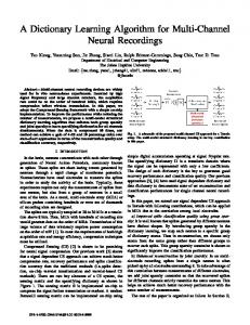
where D ( θ, θ 0 ) denotes the function distortion between subregion θ 0 and θ , C ( θ ) the complexity of the subregion θ and ζ ∈ [0,∞[ defines the sharpness rate of the kernel. 3. Algorithm evaluation In this part, we test our model with a simple mathematical function modelization, chosen to highlight specific properties. Let F be the function from R2 to R: F ( x, θ ) = θe

2

2

–( θ + x )

where

θ ∈ [ – 2, 2 ] ;x ∈ [ – 2, 2 ]

F

x θ fig. 1: F( θ ,x) function

(see fig. 1)

We have chosen, for this simple example, a deterministic way (not optimal) to cut up the Θ space: this function is divided in 41 subregions along the θ axe (step 0.1). For each subregion θ = { – 2, – 1.9, – 1.8, ...1.9, 2 } we take one NN (a 1x2x1 MLP with one bias neuron in first layer) fed with x ∈ [ – 2, 2 ] . The LCL Algorithm is applied on these multi MLP architecture with the following kernel: h ( ζ, D ( θ, θ 0 ), C ( θ ) ) = e

– ζD ( θ, θ 0 )C ( θ )

(3)

where D ( θ, θ 0 ) = θ 0 – θ (Euclidean distance) and C ( θ ) = – ln ( p ( θ ) ) whith p ( θ ) is the probability of the subregion θ (subspace energy function). h(.)

ζ = 2.5 θ0 = –1

θ

fig.2: example of kernel h ( . ) To enlighten the importance of the additional term of the lateral contribution in the backpropagation learning algorithm, we test our model with different kernels (3) by changing the ζ values from 2.5 (too small values lead to chaotic behavior). The fig. 3-4 show, for ζ → ∞ (BPA) and ζ = 2.5 (LCLA), the error vs θ (41 NNs) and epoch (120 epochs). θl

epoch

θl

θ

epoch

θ

fig. 3-4: Error(x100) vs θ (NNs) and epochs for Dirac kernel (left) and ζ =2.5 (right)

These results seem to indicate that the quickness of convergence is highly increased when the lateral contribution is employed. This point is more carefully studied below.

4. Mathematical point of view 4.1 Formalization The situation described in section 2 can be formalized in the following way: We consider a continuous family of functions { f θ(.), θ ∈ Θ } , for instance, for the distance: fθ – fθ 0

1

= sup f θ ( x ) – f θ ( x ) 0 1 x

(4)

The error between the desired output f θ and the actual one is given with a loss function l of the form: l( f , g) =

∫ λ ( f ( x ), g ( x ) )µ ( dx )

(5)

where µ is the probability distribution over the input space (or learning set). What is natural to search, is a set of connections { W (θ) } θ ∈ Θ continuous with respect to θ , ie: θ → W (θ) has to be continuous. For this purpose we define a new error function for each θ 0 by: L ( W , θ0 ) =

∫ lc ( θ – θ0 )l ( f θ ( . ), φW (θ) ( . ) ) dθ

(6)

Θ

lc ( θ – θ 0 ) is viewed as the strength of the influence of θ (the error at θ ) at the point θ0 .

Thus we have the stochastic learning algorithm (of gradient type): W t + 1 ( θ 0 ) = W t ( θ 0 ) – ε ∫ lc ( θ – θ 0 ) ∇W λ ( f θ ( x t + 1 ), φ W t(θ) ( x t + 1 ) ) dθ

(7)

Θ

where x t + 1 is chosen at random from the distribution µ , ∇W λ ( . ) is the gradient with respect to W. The O.D.E [7] describing the mean behavior of Wt writes: d W ( θ 0 ) = – ∫ lc ( θ – θ 0 ) ∇W l ( f θ ( . ), φ W t(θ) ( . ) ) dθ dt

, θ∈Θ

(8)

Θ

As soon as θ → ∇W l ( f θ ( . ), φ W t(θ) ( . ) ) is Borel-like, θ → W t(θ) is continuous. Now suppose that lc is sufficiently close to the Dirac means at 0, by a continuity argument, if W *(θ) is a continuous family of local minimum of l ( f θ ( . ), φ W (θ) ( . ) ) , it is t still a family of local minimum of L ( W , θ ) . Consequently, the learning algorithm proposed can minimize each of the l ( f θ ( . ), φ W (θ) ( . ) ) while preserving some continuity properties of W (θ) , as a funct tion of θ . This is true at least where lc is sufficiently sharp (numerical examples show that it works well even if lc is not so sharp). 4.2 Heuristic: The “intuitive” underlying idea is a sort of cooperation principle. When we update W (θ 0) , we not only use the gradient of the error at θ 0 , but we take in account the gradient of the errors of θ neighbors of θ 0 . If at θ 0 , but also at any θ near θ 0 , W t(θ 0) is at the edge of a deep well of l, it will attract all its neighbor in the well, because its

gradient is large and W t(θ) , for θ close to θ 0 is close to W t(θ 0) . On the other hand and if lc is sufficiently sharp this has no far range influence, this “cooperation principle” is only local. And the snowball effect spreads this influence from one NN to its neighbors. 5. Optimization of LCLA Of course, we can use existing optimization of the backpropagation learning algorithm [13] to increase the quickness and find the edge of a deep well of l in one θ 0 . When this edge is found we can use an algorithm, such as BFGS [9][3], to go rapidly to this local minima and then go back to the previous optimized LCL algorithm to search an other edge of a deep well of l. We can also improve it by an optimization of lc(.) kernel, by defining one kernel per connection. The heuristic of this idea is that each feature extracted by one weight in NN ( θ 0 ) could be the same for an other NN ( θ ) . So, each component of this new kernel (matrix indexed by ij) can be rewriten as: h ij ( ζ ij ( θ, θ 0 ), D ( θ, θ 0 ), C ( θ ) ) = e

– ζ ij ( θ, θ 0 )D ( θ, θ 0 )C ( θ )

(3b)

where ζ ij ( θ, θ 0 ) is the lateral contribution rate for the connection ij with regard to θ and θ 0 . This rate can be on-line adapted with regard to the comparison of W ij and the ∇W ijl ( . ) direction for each pair { θ, θ 0 } at each step, or off-line adapted with regard to the symmetries of the function F(.). This off-line adaptation can be included in the term of distortion D ( θ, θ 0 ), allowing the VQ algorithm to move two classes closer than if the term of distortion should only take the input space topology into account. 6. Conclusion The main improvements of LCL algorithm are not only the quickness of convergence of learning processing but also a new insight of the synaptic weight, showing that the behavior of a neural network in context θ 0 is directly linked to the behavior of every NNs in θ close to θ 0 . This link is due to the strong constraint that θ → W (θ) must be continuous. It is now natural to try to merge these NNs into one with synaptic weights estimated through the behavior of context θ . Accordingly, we have developed an architecture for weight estimation named OWE (Orthogonal Weight Estimator) and tested it on control problems[5]. The ongoing studies correspond to testing the LCL algorithm for more and more complex input space, and defining generalized models to embed LCLA and the on-line Vector Quantization [6].

References [1] Buhmann J., Kuhnel H.: Complexity Optimized Vector Quantization: A Neural Network Approach, in Data Compression Conference Proceedings, March 24-27, 1992, Snowbird.

[2] Buhmann J., Kuhnel H.: Unsupervized and Supervised Data Clustering with Competitive Neural Networks, in Proceedings of IJCNN’92 Baltimore IEEE Press. [3] Dennis J.E. and Schnabel R.B.: Numerical Methods for Unconstrained Optimization and Nonlinear Equations, Prentice-Hall (Ed.), 1983. [4] Guez A., Protopopescu V., Barhen J.: On the stability, storage capacity, and design of a nonlinear continuous neural networks, in IEEE Transactions on System, Man and Cybernetics, Vol 18 N 1 Jan/Feb 1988. [5] Jacobs R.A., Jordan M.I., Nowlan S.J., Hinton G.E.: Adaptative Mixtures of Local Experts, in Neural Computation, 3, 79-87, 1991. [6] Kramer A. H., Sangiovanni-Vincentelli A.: Efficient Parallel Learning Algorithms for Neural Networks, in D. S. Touretzky (ed.), Advances in Neural Information Processing Systems 1, Morgan Kaufmann. 1989. [7] Kushner H.J, Clarck D.S.: Stochastic Approximation for Constained and Unconstained Systems, in Applied Math. Science Series, 26, Springer, 1978. [8] LeCun Y.: Procedure d’apprentissage pour réseaux à seuil asymétrique, Proceedings of Cognitiva 1985, Paris. [9] Minoux M.: Programmation mathématique, Bordas et CNET-ENST., Paris,1983,1989. [10] Moody J.: Fast Learning in Multi-Resolution Hiearchies, in D. S. Touretzky (ed.), Advances in Neural Information Processing Systems 1, Morgan Kaufmann. 1989. [11] Pican N., Alexandre F.: Integration of Context in Process Models Used for Neuro-Control, in IEEE SMC’93 Conference. Le Touquet. October 17-20, 1993. [12] Rumelhart D.E., Hinton G.E. and Williams R.J.: Learning internal representations by error propagation, in Parallel Distributed Processing: Explorations in the Microstructures of Cognition, Vol.1,MIT Press, pp. 318-362. 1986. [13] Schiffmann W., Joost M., Werner R.: Optimization of Backpropagation Algorithm for Training Multilayer Perceptron. in ESANN 93 Proceeding. Bruxelles 1993. [14] Silva, Fernando M. and Almeidia, Luis B. : Speeding up Backpropagation, Advanced Neural Computers, Eckmiller R. (Editor), page 151-158, 1990.