A Multi-Objective Evolutionary Algorithm for Portfolio Optimisation No¨el-Ann Bradshaw and Chris Walshaw and Constantinos Ierotheou and A. Kevin Parrott 1 Abstract. The use of heuristic evolutionary algorithms to address the problem of portfolio optimisation has been well documented. In order to decide which assets to invest in and how much to invest, one needs to assess the potential risk and return of different portfolios. This problem is ideal for solving using a Multi-Objective Evolutionary Algorithm (MOEA) that maximises return and minimises risk. We are working on a new MOEA loosely based on Zitzler’s Strength Pareto Evolutionary Algorithm (SPEA2) [20] using Value at Risk (VaR) as the risk constraint. This algorithm currently uses a dynamic population in order to overcome the problem of loosing solutions. We are also investigating a dynamic diversity and density operator.
1
Introduction
Allocating one’s assets optimally in a portfolio is the goal of every investor. Much of the theory of portfolio optimisation is detailed in Markowitz [17]. Investors need to balance the objective of maximising the return on their investment with the constraint of minimising the risk involved. It is generally accepted that the greater the expected return, the greater the risk. Volatility is the standard measure of risk used by Markowitz and others but the drawback to this approach is that volatility is the measure of share price fluctuation without reference to direction. Thus we propose to use VaR as the measure of risk. Portfolio optimisation problems can be shown to be NP-Hard [10] and thus heuristic algorithms are a typical way to address them. Gilli and K¨ellezi [14] used Threshold Accepting and Maringer [16] classifies a number of other single-objective heuristic algorithms. Typically these approaches aim to maximise the return with the constraint that the risk should not be above a given level. This paper, alongside work by Arma˜nanzas and Lozano [4] and Chiam et al. [8], recasts the problem with a multi-objective approach where the maximisation of return and minimisation of risk are treated as two separate objectives. These are then combined into a single fitness function with each objective given equal weighting. The use of a multi-objective algorithm allows several solutions to be produced for the same problem but with different attributes [11]. Thus at a glance it is possible to see how much return one gains in comparison to the level of risk incurred. With large complex portfolios this seems to be a promising approach to investigate and we propose using a MOEA similar to SPEA2 to address it. The rest of this paper is organized as follows: section 2 recounts the background behind portfolio management and the various measures of risk, section 3 looks at optimisation methods such as multiobjective and genetic algorithms, section 4 describes our algorithm, 1
University of Greenwich, UK, email:
[email protected]
section 5 presents our results and finally, section 6 provides the conclusion.
2
Portfolio Management
2.1
Background
Portfolio management is concerned with choosing shares that will yield the best return over a given period of time. Markowitz [17] shows that a wide diversification of shares will tend to give the maximum return with the least amount of risk because shares from similar companies might behave in the same way, yielding similar risks and returns at similar times. If there is diversification in the portfolio then it is less likely to have periods of high return followed by periods of high risk. It is important to note that the risk of the overall portfolio (the combined assets) is less than the average risk of the individual assets. Markowitz’s model of portfolio optimisation provides a detailed algorithm that maximizes the return and minimises the risk. However, this model is impractical when looking at large numbers of assets. Thus alternative approaches need to be sought.
2.2
Risk Measures
Risk can be used to represent what is unknown about a portfolio. In this context it can mean the chance of the value of the shares decreasing or increasing. Traditionally the measurement of risk used is volatility. Volatility is the measure of how the value of the asset changes and can thus be positive or negative depending on price movement. This paper uses risk purely as a negative measure. In other words what could go wrong and how much can be lost or ‘how bad can things get?’ [15] There are a number of different ways of determining risk; we consider the Value at Risk approach.
2.2.1
Value at Risk
VaR was recommended as the appropriate measure of financial risk by the Basel Accord Amendment [1] in 1996 and has been heavily promoted by J.P Morgan in RiskMetricsTM Technical Document [2]. Since then it has become widely used by banks, securities firms, commodity merchants and other trading organisations. According to RiskMetricsTM [2], ‘VaR is a measure of the maximum potential change in value of a portfolio of financial instruments with a given probability over a pre-set horizon’. Its popularity is due to it being easy to understand: it reduces the level of risk to a single number which can be easily compared. Hull
[15] shows this clearly; for example it might be stated that a particular portfolio has a 1-day VaR of $1 million at the 99% confidence level. This means that there is a 1% chance that the value of the portfolio will decrease by $1 million or more during one day. However it has drawbacks; the major one being that it assumes the share price returns follow a normal distribution which is not always accurate and may result in the risks being under-estimated [16]. For this reason it is probably advisable to also look at Conditional Value at Risk (CVaR), also known as Expected Tail Loss (ETL) and Expected Shortfall (ES), which is the expected risk in the worst x% of cases (see below). VaR describes the expected loss of a portfolio with a given probability. There are three main ways to calculate it, this paper uses the simplest and most usual method: the variance covariance approach.
2.2.2
Variance Covariance Method
As the name suggests this method involves constructing a large covariance matrix of all the assets using data from the variances. It is the approach used in RiskMetricsTM [2]. The variances can be computed using a variety of methods including historic volatility, EWMA and GARCH (1,1) which are detailed by Hull [15]. The main assumption that has to be made in order to compute this method is that the risk factor returns are normally distributed. This is equivalent to saying that over a period of h days we have profit / loss of ∆Rt = Rt+h − Rt (1) where Rt indicates the return at time t and ∆Rt the total change, i.e. profit or loss over this period then, ∆h Rt ∼ N (µ, σt2 )
(2)
In other words over h days the returns follow a normal distribution with mean µ and standard deviation σ. To compute VaR for a portfolio we take the covariance matrix C of all the assets and the vector of weights v. Using the following formula we find the variance σt2 . p σt = (v 0 Cv) (3) This in turn allows us to compute VaR using the Z values from the tables for the normal distribution: VaR = Zα σt
(4)
Values for Z will change depending on the chosen value for α. It is usual to take α = 5% but this can vary depending on which level of confidence one uses.
2.2.3
Conditional Value at Risk
CVaR can be considered to be an extension of VaR. The problem with the VaR model described above is that the value in the tail might be higher than anticipated. CVaR was introduced by Artzner et al. [5]. Whereas VaR finds the minimum level of loss that can be expected, CVaR finds the expected or average loss, given that a loss has occurred. Thus the value of CVaR will be at least as large as VaR and often larger, informing investors the extent of the risk [3]. Although CVaR is not used in this paper, its usefulness as a measure of risk will be investigated as part of the further work.
2.3
Summary
This section has provided some of the background information on portfolio management in connection with calculating risk.
3
Optimization Methods
Heuristic optimisation methods are necessary where problems are NP-hard and would take an unreasonable amount of computational time to solve exactly [16].
3.1
Evolutionary Algorithms
The Genetic Algorithm (GA) was first developed by John Holland in the 1960’s [6]. It uses the process of Natural Selection to find the optimal solution through a series of populations that combine and mutate solutions until the optimal is reached. Different optimisation problems require different methods of mutating and combining solutions. GAs come under one branch of ‘nature inspired’ heuristic algorithms that are known generally as Evolutionary Algorithms (EAs). EAs allow for more flexibility than following exactly gene-based rules and can, for example, accommodate more than one objective function [11]. One of the key aspects of the EA is identifying the fitness function. The level of fitness of a solution determines whether that solution remains in the population or not. Thus the fitness function must accurately describe the objective.
3.2
Multi-Objective Evolutionary Algorithms
A major difference between single-objective optimisation and multiobjective optimisation is that in the former we obtain a single solution and in the later we have a number of non-dominated solutions [11]. If both objectives are of equal importance it is not possible to say which solution is best as there is always a trade-off between a solution being good for one objective and less good for another. However if one is of greater concern than another it might be more obvious which solutions are best. The use of MOEAs began with David Schaffer’s thesis in 1984 [18] which suggested a way to use a GA to capture multiple trade-off solutions. These have been adapted and since the mid-1990’s have been used more widely including areas such as scheduling and routing problems, and finance and economics [11]. General applications of MOEAs have been surveyed by Coello Coello and Lamont [9] and more specifically within the area of finance by Castillo Tapia and Coello Coello [7]. MOEAs present the user with a range of solutions that they can then choose from. For example with portfolio optimisation there will be some solutions with a high rate of return and a high risk and others with a low risk and a low return. Thus an investor will have to decide what sort of trade-off between risk and return they are prepared to accept. The solutions produced by a MOEA are usually bounded by a curve, known as the Pareto-optimal front. The solutions lying on this curve are known as Pareto-optimal solutions [11]. There are several well documented and tested MOEAs [12] [20]. Some of these have also been used to solve the Portfolio Optimisation problem. Skolpadungket et al [19] found that SPEA2 out-performed other algorithms. Our proposed algorithm is loosely based on SPEA2 but incorporates a dynamic population in order to include all nondominated solutions as well as the highest ranked solutions.
3.3
Summary
This section has outlined the importance and basics of evolutionary heuristic optimization methods.
4 4.1
18
5
Method
5
We are working on an algorithm which uses a dynamic diversity operator. Currently however, the code is in prototype form and to date only a dynamic population mechanism has been incorporated. Portfolio optimisation seeks to maximise the portfolio return and minimise the risk. In order to implement this we need to either maximise the return and negative risk or conversely minimise the risk and negative return. This is known as the Duality Principle and is discussed in Fryer [13]. The algorithm selects combinations of different weights of different assets and allocates them to a portfolio. It computes the total return of this portfolio and the portfolio VaR and then sorts solutions with regard to their fitness. Return is calculated by: n X
w j rj
18
6
12
16
3
14
(6)
where ||Ri || is the total normalised return and ||Vi || is the total normalised risk. To avoid losing Pareto-optimal solutions which (under this criteria) might not be the fittest solutions, the solutions are also sorted into dominated and non-dominated arrays based on their values both for total return and also for VaR. If necessary, the population is then increased each generation to include all non-dominated solutions. The number of mutations and combinations is also increased as a percentage of the entire population. Because this algorithm is multi-objective there is no one solution but a range of possible solutions. The ‘best’ one will depend on whether an investor wants to obtain maximum return which will have a higher risk or wants to decrease risk and take a lower return.
Crossover Operator
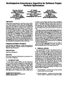
The problem of portfolio management necessitates a different process for combining and mutating solutions. The weights of the shares in the portfolio are the variables that are being subjected to change in these processes. It is necessary to ensure that the total weight is kept the same. This is not easy to do with a conventional combination method so a new combination algorithm that allows for a small mutation has been designed. This means that two different weight solutions combine but then a random weight is mutated to ensure that the total weights add up to the same amount. The example in Figure
12
4
13
14
9
16
3
6
Combination 2 before reallocation (total weight 52) 5
12
4
15
14
Combination 1 after reallocation 18
9
16
1
6
Combination 2 after reallocation
(5)
where wj is the weight of each asset and rj is the return associated with each asset. Risk is calculated using VaR as in equation 4 with α = 5%. Currently the solutions chosen to remain in the population are computed by sorting the population to a single valued fitness function. This fitness function consists of taking the normalised value of the portfolio return less the normalised value for the portfolio VaR. They are then sorted and the fittest ones saved into the population for the next generation.
4.2
13
Combination 1 before reallocation (total weight 48)
Figure 1. Example of the combination algorithm
j=1
Max||Ri || − ||Vi ||
4
Parent 2
A MOEA for Portfolio Optimization
Ri =
9
Parent 1
1 helps to illustrate this. Here we are taking the total weight as 50 and only using five assets. This shows that combination 1 and 2 are initially formed of weights taken randomly from parent 1 and 2. This will mean that the total weight does not add up to 50. So another of the weights is chosen at random and an amount is either removed or added as appropriate. The code will also choose multiple weights at random in the case where the first weight chosen is not sufficient to re-balance the total weight of the combination. This is in contrast to the crossover operation described in Chiam et al. [8]. Here only one solution is used in the operation and only the order of the weights is changed. This would seem to limit the diversity of the population.
4.3
Mutation Operator
A separate mutation operator is also needed to ensure that the population is as diverse as possible and thus a large part of the solution space is examined. This operator takes the weights and identifies one to mutate at random. A random percentage change is subtracted from this random weight. Another random weight is selected and this change is added to it thus ensuring that the total weight is kept the same. In Figure 2 we have an example of the algorithm selecting a vector of weights at random. It then chooses a non-zero cell at random, the third cell in the above example. It calculates a percentage of this and returns a whole number, which in this case is 7. This amount ‘7’ is taken off the first cell and then added to another random cell which in this example is the last one. This again differs from Chiam et al. [8] as their algorithm swaps two cells rather than adding and subtracting a random amount. We believe that our approach increases diversity, something that is necessary in these algorithms.
2
19
15
4
10
8
4
17
The algorithm was run several times using varying values for the initial population size (50,100 and 500) and number of generations (from 100 to 1000). The initial number of mutations and combinations were set as 50% of the initial population and then grew as the population increased. The confidence interval for VaR was kept at 5% but can be altered, as can the total weight of the portfolio. The greater the initial population and the more generations that were run the longer the computational time. However, although numbers of solutions increased, the general span of the non-dominated solutions and the Pareto-optimal curve remained approximately the same.
Random
2
19
Mutation
Figure 2.
Example of the mutation algorithm
5.2
Results 25
Summary
20
This section details the changes required between a standard MOEA and the one used in relation to the specific problem of portfolio optimisation.
5
Value at Risk
4.4
10
5
Preliminary Results
5.1
15
0
Test Bed
0
50
100
150
200
250
300
350
400
Total Return
In order to test the MOEA we have set up a case study with a limited number of shares. Ultimately we would hope to use all the shares in the S&P100 index and create an algorithm that picked those with the best investment potential. This case study uses the assets shown in table 1. The final work will use further test data from several exchanges.
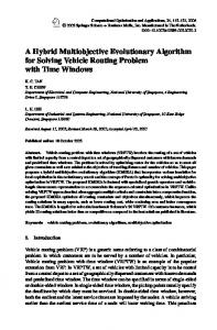
Figure 3. Results using an initial population of 50 with 200 generations
Table 1. Table to show assets used by name and S&P abbreviation 25
Abbreviation C KO BAC F GE AAPL IBM ORCL MAC XRX WMT RF PG PFE MSFT MMM HPQ JPM DELL DIS
The MOEA was run with data from these assets between January 2000 and December 2006. This period was chosen as it was also used for our previous work on EAs for finding trading rules and research into volatility in the emerging market using assets from the stock exchange in Mauritius.
20
Value at Risk
Name Citigroup Inc Coca Cola Co (The) Bank of America Cp Ford Motor Co General Electric Apple Inc International Business Machines Oracle Corp McDonald’s Cp Xerox Cp Wal-Mart Stores Inc Regions Financial Cp Procter and Gamble Co Pfizer Inc Microsoft 3M Company Hewlet Pacard Co JP Mporgan Dell Inc Walt Disney-Disney Cp
15
10
5
0 0
100
200
300
400
500
Total Return
Figure 4. Results using an initial population of 50 with 500 generations
We can see in Figure 3 that we have a reasonably diverse population. The lowest VaR value of 3.7 corresponds to a return of 86, whereas to obtain a higher return of 338 a considerably higher risk of 20.6 is incurred. Although there are a greater number of solutions in Figure 4 there is little change except that there are now an increased
number of solutions lying on the Pareto-front. There are also more solutions with a high return and high risk measurement. Maximum return is now 381 and maximum risk 23.6.
20
25
15
20
Value at Risk
Value at Risk
25
When the algorithm is run using an initial population of 500 we obtain a similar solution to Figure 6 but now with only 200 generations. We have a maximum return of 393 corresponding to a maximum return of 21.6 and a minimum return of 102 corresponding to VaR of 3.6.
10
5
15
10
0 0
50
100
150
200
250
300
350
5
400
Total Return 0 0
100
200
300
400
500
Total Return
Figure 5. Results using an initial population of 100 with 200 generations Figure 7. Results using an initial population of 500 with 200 generations
25
800
20
Time (seconds)
Value at Risk
700 15
10
5
600 500
100
400
50
300
500
200 100
0 0
100
200
300
400
500
Total Return
0 0
500
1000
1500
Number of Generations
Figure 6. Results using an initial population of 100 with 500 generations
Increasing the number in the initial population makes little difference to the results except to effect the amount of time the algorithm takes to run. It can be seen in Figure 8 that there is not much difference in computational time between initial populations of 50 and 100 (merely a matter of seconds) but this lengthens considerably when increased to 500. Final population sizes are also vastly different as can be seen in table 2. Table 2. Table to show final population size when running the algorithm for 200 generations for different initial population sizes. Initial Population Size 50 100 500
Final Population Size 4366 10084 36786
Figure 8. Graph to show how the computational time increases relative to the number of generations used with initial population sizes of 50, 100 and 500.
This test case indicates that using a dynamic population means that a small initial population size has little effect on both the results produced or the run-time. The run-time increases considerably with a large initial population and the results are not significantly improved. Obviously the number of generations also has an effect on the runtime but with a small initial population this is fairly small. The results show that the algorithm manages to produce very good results with only 200 generations after only a short amount of time; additional generations improve the result slightly, but perhaps not significantly. In order to examine this further a new test bed was put together using data from the same companies but this time from 1990-1999. This provided an increased amount of data. The results were very similar although took longer with the increased quantity of data. The
Pareto-optimal front took slightly longer to reach but once reached (500 generations with initial population of 100) it was left unchanged with successive generations. Interestingly when making comparisons between run-time, number of generations and initial population, a similar graph (Figure 9) is obtained to the previous one. This suggests that using a dynamic population means that one only has to use a small initial population in order to achieve the Pareto-optimal front rather than use a larger initial population size where convergence takes longer. 1400 1200
Time (seconds)
1000 50
800
100 600
500
400 200 0 0
200
400
600
800
1000
1200
Number of Generations
Figure 9. Graph to show how the computational time increases relative to the number of generations used with initial population sizes of 50, 100 and 500 and an increased quantity of data.
The final version of the paper will seek to establish the veracity of this conclusion with additional test cases and results.
5.3
Summary
This section has given examples of some of the preliminary results that have been obtained running this algorithm with different parameters.
6
Conclusions
This paper has shown that using a MOEA to allocate the optimal number and quantity of shares into a portfolio is worthy of consideration and could provide useful information for investors. Preliminary results show a diverse set of solutions ranging from high return and low risk to the opposite. We are currently investigating a dynamic diversity and density operator but the work is not sufficiently developed to report on.
6.1
Future Work
Our main investigation is concerning how to preserve diversity. In terms of the result, future work will be carried out on testing the algorithm against other known algorithms and making comparisons using test data. Investigations into how to preserve diversity using density measures will also be looked at. Future work concerning portfolio optimisation will include looking at different ways of calculating volatility for VaR. Other risk measures will be examined and may be incorporated into the algorithm as a third objective function. Further
investigations will also be made with other data sets and different time periods.
Acknowledgment This work was supported in part by a bursary from the University of Greenwich, London, UK.
REFERENCES [1] Amendment to the capital accord to incorporate market risks. Basle Committee on Banking Supervision, Jan 1996. [2] Riskmetrics - technical document. JPMorgan/Reuters, Dec 1996. [3] C. Alexander, Market Models, John Wiley and Sons LTD, Chichister, UK, 2001. [4] R. Armananzas and J. A. Lozano, ‘A multiobjective approach to the portfolio optimization problem’, Technical report, ISG - Department of Computer Science and Artifical Intelligence, (2005). [5] P. Artzner, F. Delbaen, J.-M. Ebner, and D. Heath, ‘Coherent measures of risk’, Mathematical Finance, 9, 203–208, (1999). [6] R. J. Bauer, Genetic Algorithms and Investment Strategies, John Wiley and Sons LTD, New York, USA, 1994. [7] M. G. Castillo Tapia and C. A. Coello Coello, ‘Applications of multiobjective evolutionary algorithms in economics and finance: A survey’, in IEEE Congress on Evolutionary Computation, pp. 532–539, (Sept 2007). [8] S. C. Chiam, K. C. Tan, and A. Al Mamum, ‘Evolutionary multiobjective portfolio optimization in practical context’, International Journal of Automation and Computing, 05(1), 67–80, (January 2008). [9] C. A. Coello Coello and G. B. Lamont, Applications of Multi-Objective Evolutionary Algorithms, World Scientific, Singapore, 2004. [10] J. Danielsson, B. N. Jorgessen, C. G. Vries, and X. Yang, Optimal Portfolio Allocation under a Probabalistic Risk Constraint and the Incentives for Financial Innovation, Ph.D. dissertation, London School of Economics, June 2001. [11] K. Deb, Multi-Objective Optimization using Evolutionary Algorithms, John Wiley and Sons LTD, Chichister: UK, 2001. [12] K. Deb, A. Pratap, S. Agarwal, and T. Meyarivan, ‘A fast and elitist multi-objective genetic algorithm: NSGA-II’, Technical report, Indian Institute of Technology Kanpur, (2000). [13] M. J. Fryer and J. V. Greenman, Optimisation Theory - Applications in O.R. and Economics, Edward Arnold, 1987. [14] M. Gilli and E. K¨ellezi, Computational Methods in Decision-Making, Economics and Finance, chapter A Global Optimization Heuristic for Portfolio Choice with VaR and Expected Shortfall, 165–181, Kluwer, 2001. [15] J. C. Hull, Options, Futures and Derivatives, Prentice Hall International, New Jersey, USA:, 6th edn., 2006. [16] D. Maringer, Portfolio Management with Heuristic Optimization, Springer, 2005. [17] H. M. Markowitz, ‘Portfolio selection’, The Journal of Finance, 1(7), 77–91, (March 1952). [18] J. D. Schaffer, Experiments in Machine Learning Using Vector Evaluated Genetic Algorithms, Ph.D. dissertation, Vanderbilt University, Nashville, TN, USA, 1984. [19] P. Skolpadungket, K. Dahal, and N. Harnpornchai, ‘Portfolio optimization using multi-objective genetic algorithms’, in IEEE Congress of Evolutionary Computation, (2007). [20] E. Zitzler, M. Laumanns, and L. Thiele, ‘SPEA2: Improving the strength pareto evolutionary algorithm’, Technical report, Swiss Federal Institute of Technology (ETH) Zurich, (2001).