vacuum cleaner platform [1] or a health care robot [2]). Today there are some techniques for solving SLAM with reasonable complexity [3] (ex. real-time particle ...
A Lightweight SLAM algorithm using Orthogonal Planes for Indoor Mobile Robotics Viet Nguyen, Ahad Harati, Roland Siegwart Autonomous Systems Laboratory Swiss Federal Institute of Technology (ETH Zurich) R¨amistrasse 101, CH-8092 Z¨urich, Switzerland Email: {viet.nguyen, ahad.harati, roland.siegwart}@mavt.ethz.ch Abstract— Simple, fast and lightweight SLAM algorithms are necessary in many embedded robotic systems which soon will be used in houses and offices in order to do various service tasks. In this paper the Orthogonal SLAM algorithm is presented as an answer to this need. In continuation of our previous work, the algorithm is extended to generate 3D maps and empirically validated by mapping the long corridor of our lab with the accuracy comparable with hand measured ground truth. The main contribution resides in the idea of reducing the complexity by using orthogonality constraint in indoor environments. This is done by mapping only planes that are parallel or perpendicular to each other which represent the main structure of most indoor environments. Having this assumption, we use an inclined sensor setup (fixed 2D SICK laser range finders) to generate 3D orthogonal maps. The algorithm is extremely fast since in each step it just processes one line of laser measurements.
I. I NTRODUCTION One of the most basic behaviors of an intelligent mobile robot is autonomous navigation. This capability is realized by obtaining a suitable representation of the robot surroundings, which is called mapping. Simultaneous Localization and Mapping (SLAM) is a complex case where the robot is also required to remain localized with respect to the portion of the environment that has already been mapped. Regardless of the innate complexity, SLAM algorithms are eventually needed in simple embedded mobile robots with limited processing power. Many of them are targeted for indoor usage as medical or housekeeping applications (see for example a vacuum cleaner platform [1] or a health care robot [2]). Today there are some techniques for solving SLAM with reasonable complexity [3] (ex. real-time particle filters, submapping strategies or hierarchical combination of metrictopological representations). However, these techniques are developed having powerful computational resources in mind. Less research effort has already been spent on development of lightweight SLAM algorithms which are of vital importance in many applications of mobile robotics. Considering indoor environments, in this paper we aim to develop a lightweight and real-time consistent SLAM algorithm based on planar surfaces which are the dominant structures. In our previous work we presented OrthoSLAM [4] for realtime mapping of office-like environments. Considering a very common constraint usually present in many indoor environments, the orthogonality, we showed that the uncertainty on the robot orientation can be kept bounded and
knowing the robot orientation, SLAM is reduces to a linear estimation problem. The simple assumption of orthogonality on shape of the environment, comes from the fact that in most indoor engineered environments, major structures, like walls, windows, cupboards, etc., can be represented by sets of lines or planes which are parallel or perpendicular to each other. For reconstruction of the desired map, it is sufficient to extract and maintain those major features. In fact, ignoring other lines/planes (arbitrary oriented or non-orthogonal) not only does not lead to loss of valuable information, but also brings amazing robustness on the robot orientation and filter out many dynamic objects. The assumption of orthogonality as a geometrical constraint has already been used by some other researchers, for example [5], [1]. This geometrical constraint is usually applied as a post-processing step in order to increase the precision and consistency of the final map. However, in our approach the orthogonality assumption is not applied as an additional post-processing constraint, rather it is used to select only orthogonal lines as observations. In the orthogonal framework, lines and planes are represented by just one distance parameter (no orientation is needed), hence each line directly provides some information on corresponding plane, which is then accumulated in a Kalman Filter. The mapping is performed based on this constraint and in a simplified framework, rather than applying the constraint as an extra observation afterward. This is a great difference which leads to the removal of non-linearities in the observation model and rather precise and consistent mapping. In this sense our work is similar to Orthogonal Surface Assignment, the very recent work of Kohlhepp et al. [6]. Their approach is using the same constraint in the framework of multi-hypothesis tracking. However, we construct orthogonal planes from 2D observations and the whole infrastructure of our algorithm is much simpler and faster. The main difference between the work presented here and majority of the existing efforts in the literature relies in the way the complexity is reduced. While the other approaches modify the basic algorithm by some assumptions and approximations, we propose to use a constraint of the environment. This allows keeping a complete coherent approach that now is actually applied to a simplified problem. This results in a better performance for all cases that do not violate the orthogonality assumption.
To build 3D maps of the environment, apart from stereo cameras which deliver range information just for textured part of the scene, usually 3D laser scanners are used. These 3D scanners are usually constructed by rotating a 2D laser range finder. This can be implemented by nodding, stepwise or continuous rotation around lateral or radial axis (see [7], [8], [9], [10], [11], [12]). This common approach provides rich point clouds which can be used to generate detailed 3D maps of the environments. However, not always obtaining a lot of information is necessary or even useful. The first problem in such cases is the stop and move scenario which is normally mandatory to obtain consistent 3D observations. That is inconvenient and sometimes not practical. Another serious problem is how to segment huge amount of points into homogeneous regions with reasonable performance. An alternative approach is to keep the 2D observations and generate 3D data by the movement of the robot itself. Usually a horizontally mounted SICK is used for 2D localization and another vertically mounted SICK accumulates rows of points in 3D in order to do the mapping (see [13], [14], [15], [16], [17]). Instead of using two different scanners perpendicular to each other, it is also possible to get the 3D coordinates of the scanned points by using only one scanner which is mounted in a tilted plane (Fig. 1) if we assume the planar surfaces are perpendicular or parallel to the ground plane. In fact, this assumption is approximately always true in indoor environments. Even in most complex parts, like staircases, still most of the surfaces satisfy this condition. Therefore the orthogonality constraint also simplifies sensing system and feature extraction algorithm. II. O RTHOGONAL P LANES The main idea of this work relies on the Orthogonality assumption on the environment. It brings amazing robustness and precision in the map building process. Estimation of the robot’s 3D orientation is virtually removed and mapping of the orthogonal planes is reduced to a linear estimation problem with one parameter per plane. It is important to emphasize that the Orthogonality assumption (or constraint) holds and in fact exists in most man-made environments. In this paper “Orthogonality assumption” and “Orthogonality constraint” are used interchangeably. In OrthoSLAM algorithm, only planes verifying the Orthogonality constraint will be selected and mapped, for example: walls, ceiling, windows, doors, cupboards, etc. Orthogonal planes are divided into three distinct groups XPlanes, YPlanes and ZPlanes which are perpendicular to x-axis, y-axis and z-axis, respectively. Clearly, orthogonal planes are parallel or perpendicular to each other. Within a group, the orientation of the planes is known. Thus, for each orthogonal plane it is necessary to estimate only one parameter which is the distance from the origin to the plane (i.e. x coordinate for x-planes and so on). The estimate elements in a group are statistically correlated but not correlated with elements in other groups. To extract planes from the environment, two inclined laser range finders are mounted in inclination of 45o to
Fig. 1. The BiBa robot. The two inclined SICKs at the top are mounted at 45o to the forward and backward direction.
Fig. 2. Orthogonal plane construction from 3D line segments. Lines 1, 3, 6, 8, 9 make up five x-planes. Lines 2, 4, 5, 7 are perpendicular to both y-axis and z-axis and thus can be only classified by comparing with already mapped planes or merging with non-associated line segments.
the forward and backward direction as shown in Fig. 1. 2D line segments are extracted from the scans (in sensor 2D frame) and transformed into the robot 3D coordinate frame. For each 3D line segment, one orthogonal rectangular planar patch is constructed by using the line segment as its diagonal. Obviously rectangular planar patches can not represent complex surfaces. However, main orthogonal surfaces in an office-like environments (e.g. walls, doors, ceilings, etc.) tend to have rectangular shape or compose of several small rectangular patches. Using 3D line segments as diagonals of orthogonal planar patches allows very fast and efficient plane construction. An example of orthogonal plane construction is shown in Fig. 2. There are nine line segments extracted from one observation. By using the Orthogonality constraint, five xplanes can be constructed from line segments 1, 3, 6, 8, 9. Obviously in order to do that the robot has to know roughly its current global orientation. Lines 2, 4, 5, 7 are perpendicular to both y-axis and z-axis, meaning they are either y-planes or z-planes. This ambiguity is resolved by comparing with already mapped planes or merging with notassociated lines in subsequent steps. This process will be described in the Data Association subsection. In fact, line 4 is from an office wall (y-plane), line 5 is from a door way (y-plane), lines 2 and 7 are from the ceiling (z-planes). In this example, there are not any non-orthogonal 3D lines (i.e. arbitrary lines which are not perpendicular to any axis of the global frame) to be discarded.
New 2D Raw Data
2D Line Extraction
2D Line Segments
3D Line Calculation
3D Line Segments
Orthogonalization
Corrected Planes
Rel. Dist Calculation
Rel. Geo. Filter
Estimation
Relative Map
Absolute Map
Absolute Map Construction
Selected Lines Data Association Robot Pose Robot Conf. Update
Fig. 3.
Plane Merge/Align
Planes
Functional structure of the OrthoSLAM algorithm.
In the above example, due to broken line segments, planes 8 and 9 may come from the same bigger x-plane as they have approximately the same x coordinate and locate near each other. This usually happens because of occlusion or openings. Thus it is a good idea to represent them as two sub-x-planes from the same big x-plane so that the number of parameters (one parameter per big plane) to estimate can be reduced significantly. The OrthoSLAM implements this two-levels of plane features so that each orthogonal plane (plane level 1) consists of several near and aligned sub-planes (plane level 2). The number of parameters to be estimated is the number of planes level 1. In this work, plane boundaries are not estimated statistically as they do not have effect on the precision of the map. Plane boundaries are only used in the data association. A simple technique for correcting plane intersections (corners) is implemented in OrthoSLAM which will be briefly described in the next section. III. T HE OrthoSLAM A LGORITHM In continuation of the previous work (see [4]), the OrthoSLAM algorithm performs 3D mapping using only orthogonal planes. The horizontal ground assumption directly implies that it is sufficient to use the 2D modeling to represent the robot pose, i.e. (xR , yR , θ). In fact, including z direction in the mapping does not improve the precision of the 2D elements of the resulting map. However, having z elements in the estimates makes the data association much more robust and also results in a complete 3D map which is a closer representation of the reality. The planes are constructed from line segments extracted from two inclined laser scanners. As already mentioned above, each orthogonal plane is represented by one parameter which is the perpendicular distance from the origin to the plane, i.e. x coordinate for a x-plane, y coordinate for a yplane and z coordinate for a z-plane. From now on we denote this coordinate as plane coordinate. The OrthoSLAM algorithm implements the relative mapping approach where the estimate elements are the relative distances between planes in the same group. This mapping approach has been shown in [18], [19], [4] to have very good consistency property for map building. Fig. 3 shows the working structure of the OrthoSLAM algorithm. It consists of several connecting modules which
will be described in the following subsections. Some of the modules work with projections of the x-planes, y-planes on the xy plane. They are implemented similarly to those explained in [4] and thus will be briefly explained. 2D Line Extraction Line segments are extracted online from raw 2D laser range scans coming from the two inclined SICKs. For this task, the Split-and-Merge algorithm is selected among other line extraction algorithms (see [20]). In this implementation, only line segments having length from 30cm are considered. 3D Line Calculation This module performs the 2D to 3D transformation of the extracted 2D line segments into the robot frame. The transformation of the segment end points is directly derived from the configuration of the inclined sensors. Data Association (DA) This module decides the matching for a new observation. The first step is to divide the new 3D segments into groups. This can be done easily by using the coordinates of the two end points. For example, an x-plane’s diagonal should have approximately equal x coordinates of the two end points. An ambiguity may happen when two pairs of coordinates are approximately equal, e.g. both x and z coordinates are approximately equal. In this case, the segment is stored in WaitList which will be analyzed and merged with other lines or planes later on. If a line segment is not parallel to any of the xy/yz/xz planes, or not orthogonal, it is discarded. Once the types of new lines have been determined, the matching with the existing planes is performed (see [4]). The overlapping is determined based on the overlapping distances in x and z directions for x-planes; y and z directions for y-planes; x and y directions for z-planes. If two planes approximately align and overlap, they are matched. Once a plane has been matched (first level), the association is also performed in the sub-plane level. At this level however it is much simpler as the decision is made based on only the overlapping distances over the two dimensions. The concept local view (as used in [4]) is also implemented in OrthoSLAM to reduce the complexity of this module to constant time. Orthogonalization The functionality of this module is, using the Orthogonality
constraint, to locally correct the constructed orthogonal plane parameters in a new observation after the data association. Due to noise and imperfect orthogonality of the environment, extracted 2D line segments (thus predicted orthogonal planes) are not perfectly orthogonal and may be slightly deviated. For the x-planesand y-planes, the projections on the xy plane of the 3D line segments are first computed. Next, the projections are rotated on the xy plane around their midpoints so that they are perfectly orthogonal to each other as described in [4]. The 3D line segments are then rotated around their centering vertical axis by the same correction angle of their corresponding projection. For z-planes, the 3D line segments are rotated around their mid point so that the resulting segments are parallel to the xy plane. Recall from [4] that the orthogonalization is independent of the robot pose. It is obvious that the corrected lines are mutually correlated after the orthogonalization, however we do not consider the correlation as an approximation. Calculation of Relative Distances between Planes This module computes the relative distances between planes in the new observation. The implementation is similar to that described in [4]. For z-planes, the distances are between the ground (the xy plane) and the z-planes. Estimation This module performs the estimation of relative distances independently for three groups x-planes, y-planes and zplanes. The estimation is a linear problem. The implementation follows the one described in [4]. Since the elements in each group are correlated, the complexity is cubic. One can optimize this operation from the fact that the covariance matrix is very sparse. However it is out of scope of this paper. Absolute Map Construction The absolute map is constructed from the estimate of the distances (the relative map) and one given x-plane, y-plane and the ground plane. The time complexity of the construction is linear on the number of planes. In this implementation, the plane boundaries are the union of those extracted in each observation. It is the future work that plane intersections (corners) will be detected so that plane boundaries will be accurately computed. Robot Configuration Update In principle, the relative mapping approach does not use the robot configuration in the estimation. The odometry information is used only in the DA process and in the case when there are not enough observed features. In a normal situation, the robot pose is computed using the updated map after the observation has been fused. Merge/Align Planes When two planes of the same group approximately align (i.e. having approximately equal plane coordinate) and they are overlapping or near each other, the planes are merged into one big plane. Their list of sub-planes are appended and
merged if overlapping. Fig. 4 shows an example of three planes (top view) where plane P 2 and P 3 align and close to each other. They are merged into one big plane. Additionally, the constraint d12 = d13 has to be satisfied and thus to be applied in order to enforce the relative map consistency (see next subsection). Finally, one distance either d12 or d13 is removed from the relative map. When two planes approximately align but they are not overlapping nor near each other, they are aligned perfectly to have the same plane coordinate. The alignment is accomplished by applying the constraint d12 = d13 . In this implementation, only plane merging is implemented. This module has a complexity of O(N 2 ) where N is the number of planes in a group. However it is called periodically (e.g. once every 50 observation steps) so that the computational overhead is minimal. To reduce the cost further, the module keeps track of plane pairs that have been verified for merging/alignment so that they are not checked until the next changes made to one of the planes. P1 d12
d13 P2
P3
Fig. 4. An example (top view): planes P 2 and P 3 align and near each other, thus they are subject to be merged. The constraints d12 − d13 = 0 is applied to improve the relative map consistency by the Relative Map Geometric Filter.
Relative Map Geometric Filter This module implements the Relative Map Geometric Filter - RMGF (see [19]) in order to to improve the relative map consistency. For the example above, after merging planes P 2 and P 3 the constraint d12 − d13 = 0 is to be applied. Usually the constraint involve more than two map elements depending on the size of the linking chain between planes P 2 and P 3. The number of constraints equals the number of plane merging. In vector form, we can write the constraint set as H(d) = 0. If we interpret the vector constraint as a perfect observation z = H(d), applying the Kalman Filter equation, we have: ˆ = d + K (0 − H(d)) d ˆ = P − K ∇H P P K = P ∇HT [∇H P ∇HT ]−1 where d and P are the map vector and covariance matrix of ˆ and P ˆ are the updated quantities after the relative map, d applying the constraints. Since the relative map elements are correlated, the complexity of the filter is O(N 3 ) where N is the vector size. However, this module is called only when there are constraints generated by the Merge/Align Planes module. IV. E XPERIMENTAL R ESULTS For the experiment, we use the Biba robot (http://www.asl.ethz.ch/) which is equipped with two
5
7 6
2
4
1
3
Fig. 5. The laboratory floor. Top picture is the construction drawing. Middle picture is the map built using pure odometry information and raw scans which is corrupted by the odometry drift. Bottom picture is the 2D view of the map built using OrthoSLAM algorithm (ceiling planes are not shown). The robot’s trajectory is marked on the map going from 1 to 7.
CPUs, two inclined SICK laser scanners (two horizontal SICKs are not used in this experiment). The two SICKs are mounted in inclination of 45o to the forward and backward directions as shown in Fig. 1. The robots are running a real-time operating system (RTAI Linux) with an embedded obstacle avoidance system and a remote control module via wireless network. In our experiment, we use a maximum scan range of 7.0m, an angular resolution of 0.5◦ and a sampling rate of 2Hz. We choose our laboratory floor as the testing zone which consists of a long, narrow hallway and office rooms on both sides. The floor has a map size of approximately 80m × 15m. A picture of the floor construction drawing is shown in Fig. 5. Unfortunately we do not have the metric information, therefore we have to make hand measurements between some selected reference points for the algorithm evaluation. The robot navigates along the hallway, visiting places from 1 to 7 as marked on Fig. 5, including several office rooms and making two closing loops. The average speed of the robot is about 30cm/s. The experiment is carried out during the working hours so that there are people walking around. In the whole run the robot performs more than 4200 observation steps. A 2D view of the map obtained by using the pure odometry information is shown in the middle picture of Fig. 5. One can see that the map is corrupted by the odometry drift. A 2D view of the map built using the OrthoSLAM algorithm is shown in Fig. 5. A 3D view is depicted in Fig. 6 (left picture) where the ceiling planes are not shown for
clarity. It can be seen that the shape and orientation of the built map is matched precisely with the construction drawing. It is an theoretically expected result: by using the Orthogonality constraint which holds for this environment, there is no orientation error in the estimate. Fig. 6 (right picture) shows the mapped planes of room 5 where the robot has visited. The walls, door way, ceiling and windows are mapped correctly compared to what in the reality. Notice that moving people, dynamic objects (e.g. opening doors) and lying around objects (e.g. tables, boxes) mostly do not appear in the scans since the scanners are facing 45o upwards. Otherwise, they are filtered out by the condition of minimal segment length, number of occurrences and the Orthogonality constraint. The built map has a size of 80m × 15m and consists of 50 x-planes, 66 y-planes and 19 z-planes. Obviously there are more planar surfaces in the reality. Nevertheless, the mapped orthogonal planes clearly represent the main structures of the laboratory places where the robot has visited. Furthermore, in term of memory usage, having orthogonal planes as the map features, including the associated relative map, is clearly a great advantage over the method using point clouds where millions of scan points are to be stored. The OrthoSLAM algorithm is performed on a labtop with a PentiumM-600MHz using the logged data of the experiment. In term of computational performance, the algorithm is able to run at 10Hz without any special optimization. This running speed is 5 times faster than the input data rate. Regarding the metric precision, the estimated map has a
Fig. 6. Left: A 3D view of the built map where the ceiling planes are not shown. The red curve in the middle is the estimated robot trajectory. Right: A zoomed-in picture of room 5. The planes are mapped correctly compared to what in the reality.
length of 82.59m compared to the hand measured value of 82.64m. The difference of 5cm is in the uncertainty range of hand measurements. Furthermore, we compared 20 distances between the selected planes in the resulting map with the hand measured values. The differences have a mean value of −0.8cm and a standard deviation of 3.5cm. This precision is acceptable when considering the errors of the sensors and hand measurements. The largest differences belong to the relative distances between planes whose locations rely on the odometry data (i.e. one of the two planes is not observed simultaneously with any other plane in the map). V. C ONCLUSION The paper has presented the OrthoSLAM algorithm as a simple, fast and lightweight solution to SLAM for indoor office-like environments. In continuation of the previous work, the algorithm is extended to generate 3D maps and empirically validated by mapping our 80m × 15m laboratory floor with the obtained accuracy comparable to hand measured ground truth. The main contribution resides in the idea of reducing the complexity by using the Orthogonality constraint (or assumption) existing in most indoor environments. This is done by mapping only planes that are parallel or perpendicular to each other which represent the main structure of most man-made environments. Having this constraint, we use an inclined sensor setup to generate 3D orthogonal maps. The algorithm is extremely fast since in each step it just processes one line of laser measurements. For future work, it is necessary to implement a plane intersection detection for a better corner estimation. We plan to implement at least one other 3D SLAM algorithm for the comparison purpose. It is also in our plan to extend partially the Orthogonality to outdoor city-like environments where the constraint of vertical planes holds for most buildings. ACKNOWLEDGMENTS This work has been supported by the Swiss National Science Foundation No 200021-101886 and the EU project Cogniron FP6-IST-002020.
R EFERENCES [1] P. Jensfelt, H. Christensen, and G. Zunino, “Integrated systems for mapping and localization,” in SLAM Workshop - ICRA, 2002. [2] D. Rodriguez-Losada, F. Matia, A. Jimenez, R. Galan, and G. Lacey, “Implementing map based navigation in guido, the robotic samrtwalker,” in Proceedings of ICRA, 2005. [3] S. Thrun, Exploring Artificial Intelligence in the New Millenium. Morgan Kaufmann, 2002, ch. Robotic mapping: A survey. [4] V. Nguyen, A. Harati, N. Tomatis, A. Martinelli, and R. Siegwart, “OrthoSLAM: A Step toward Lightweight Indoor Autonomous Navigation,” in Proceedings of IROS, 2006. [5] P. Newman, J. Leonard, J. Tardos, and J. Neira, “Explore and Return: Exprimental Validation of Real-Time Concurrent Mapping and Localization,” in Proceedings of ICRA, 2002. [6] P. Kohlhepp, G. Bretthauer, M. Walther, and R. Dillmann, “Using orthogonal surface directions for autonomous 3d-exploration of indoor environments,” in Proceedings of IROS, 2006. [7] J. Weingarten and R. Siegwart, “3D SLAM using planar segments,” in Proceedings of IROS, 2006. [8] A. N¨uchter, K. Lingemann, J. Hertzberg, and H. Surmann, “Heuristicbased laser scan matching for outdoor 6D SLAM,” in 28th Annual German Conference on Advances in Artificial Intelligence, 2005. [9] O. Wulf, K. Arras, H. Christensen, and B. Wagner, “2D mapping of cluttered indoor environments by means of 3D perception,” in Proceedings of ICRA, 2004. [10] D. Cole, A. Harrison, and N. Paul, “Using naturally salient regions for SLAM with 3D laser data,” in SLAM Workshop, ICRA, 2005. [11] P. Kohlhepp, P. Pozzo, M. Walther, and R. Dillmann, “Sequential 3DSLAM for mobile action planning,” in Proceedings of IROS, 2004. [12] M. Montemerlo and S. Thrun, “A multi-resolution pyramid for outdoor robot terrain perception,” in Proceedings of AAAI, 2004. [13] J. Weingarten, G. Gruener, and R. Siegwart, “A fast and robust 3D feature extraction algorithm for structured environment reconstruction,” in Proceedings of ICAR, 2003. [14] S. Thrun, W. Burgard, and D. Fox, “A real-time algorithm for mobile robot mapping with applications to multi-robot and 3d mapping,” in Proceedings of ICRA, 2000. [15] A. Howard, D. Wolf, and G. Sukhatme, “Towards 3d mapping in large urban environments,” in Proceedings of IROS, 2004. [16] Y. Lui, R. Emery, D. Charabarti, W. Burgard, and S. Thrun, “Using EM to learn 3D models of indoor environments with mobile robots,” in Proceedings of ICML, 2001. [17] D. H¨ahnel, W. Burgard, and S. Thrun, “Learning compact 3d models of indoor and outdoor environments with a mobile robot,” in EUROBOT, 2001. [18] A. Martinelli, N. Tomatis, and R. Siegwart, “Open Challenges in SLAM: An Optimal Solution Based on Shift and Rotation Invariants,” in Proceedings of ICRA’2004. [19] V. Nguyen, A. Martinelli, and R. Siegwart, “Handling the Inconsistency of Relative Map Filter,” in Proceedings of ICRA’2005. [20] V. Nguyen, A. Martinelli, N. Tomatis, and R. Siegwart, “A Comparison of Line Extraction Algorithms using 2D Laser Rangefinder for Indoor Mobile Robotics,” in Proceedings of IROS, 2005.