Abstractâ We present a system for 2D robot mapping which is entirely based on ..... by solving a linear equation system with n equations given by: BX = A, where X ..... Data set 'NIST maze'. a) Heavily misaligned input. b) alignment. (gray spot ...
2010 IEEE International Conference on Robotics and Automation Anchorage Convention District May 3-8, 2010, Anchorage, Alaska, USA
A Line Segment Based System for 2D Global Mapping Jan Elseberg
Ross T. Creed
Abstract— We present a system for 2D robot mapping which is entirely based on line segment representation of the environment. The system consists of multiple modules, i.e. scan number reduction, global scan alignment, scan merging and segmenterror filtering, which give an example of the simplicity of mid level data processing and the advanced possibilities opened by segment based design. The compact segment representation enables creation and optimization of a global pose graph for scan registration, which is the core of the mapping system. Experiments verify the applicability to real world data sets and lead to very compact maps, which represent single linear features, e.g. walls, with single line segments.
I. I NTRODUCTION AND A PPROACH The interest in robot mapping based on mid-level geometric structures like linear elements is currently growing. Compared to low-level point based algorithms, such approaches have advantages with respect to runtime, memory efficiency and simpler mid- and high-level analysis capability for preand post-processing. In this paper, we present a mapping approach which is entirely line segment based. We immediately extract line segments from single laser scans (e.g., using approaches described in [1]). An important design paradigm of the presented research is to keep the very efficient and compact data representation given by the extracted segments, without returning to the underlying points. This leads to the following advantages: First: the segment based approach captures structural information. This information goes significantly further than the information of object presence and location, contained in raw point data. Line segments combine multiple points to a single feature. This creates the properties of segment direction and feature membership. These properties, augmenting the property of object location, lead to more robust feature correspondences in the alignment process. In our approach, this allows for significant reduction of scans: the original data set, usually consisting of thousands of scans with high redundancy (segment overlap), can be reduced to a few hundred scans with minimal overlap, which however is still sufficient for the segment based algorithm to perform the alignment. Second: the segment based approach is fast. In indoor environments or urban outdoor environments, a typical scan consists of n < 20 segments of sufficient length, while the number of data points is typically one to two orders of magnitude higher. This becomes especially important when J. Elseberg is with Jacobs University, Bremen, Germany. R. T. Creed is with Saint Joseph’s University, Philadelphia, PA, R. Lakaemper is with Temple University, Philadelphia, PA.
978-1-4244-5040-4/10/$26.00 ©2010 IEEE
Rolf Lakaemper
feature correspondences between different scans have to be evaluated, which usually implies algorithms with runtime complexity between O(n log n) and O(n2 ). Third: the segment based approach is memory efficient, each line segment consists of two endpoints. Fourth: the segment based approach is precise. Segment endpoints don’t have to be adjusted to a resolution parameter, hence there are no quantization errors. Resolution parameters are introduced in grid based algorithms e.g. when occupancy grids are used to determine feature confidence, which is related to the segment merging and segment cleaning process, sections VI and VII. In its core, the scan alignment is computed using a global pose graph, containing the relative poses of all scans (of a pre-selected subset of the original scans). The pose graph is used to optimize line segment correspondences, measured by a line-segment similarity measure. Items one, two and three of the enumeration of advantages above, are the assumptions that make such a global approach feasible: in contrast to point based algorithms, the lower number of scans with lower number of features leads to a problem representation which can be handled by current computers. The system consists of the following components, which all utilize the segment similarity measure described in section III: first, the set of scans is reduced (section IV), followed by the scan alignment (section V). The alignment leads to poseoptimized single scans, which are merged to a single global map with a significantly lower number of segments (VI). Finally, a post processing step, scan cleaning, eliminates inconsistent line segments, which originate from scan errors of multiple sources (section VII). The output is a compact, segment based map of the environment. Scan selection and scan cleaning are examples of how segment based representation leads to simple, efficient and straightforward mid-level algorithms. For the core process, which is the scan alignment, the compact data representation by segments allows us to build a global graph which does not exceed a feasible size. It therefore allows globally consistent pose optimization on real world data sets. II. R ELATED W ORK [2] describes a line segment based mapping approach, which also extracts segments from single scans, and merges them to a global map. However, their alignment approach is sequential, with the known drawback of error accumulation. Additionally, since their segment handling is relatively basic; no segment weights are used, segment similarity is solely based on angular and mid-point distance. Reducing segments
3924
to their direction and mid-point is very critical, and works only if segments representing the same environmental feature, are seen from similar perspectives (our measure uses the center-point, too, but only to determine a single point on the merged segment. The actual distance computation goes further). Such a system can therefore only work with a relatively high scan density, which in turn increases the probability for higher accumulated errors. In contrast, our system is based on a more sophisticated similarity measure, which allows the usage of a more sparse data set, enabling true global pose graph optimization. Another line segment approach is described in [3]. This approach mainly focuses on detection and merging of lines. In its core, it is still point based: the point based global map is embedded into a grid, each cell is then represented by exactly two line segments. No alignment is reported. [3] focuses therefore on finding line segments in a point set, and uses the term mapping more in the sense of line finding, comparable e.g. to [4]. There are numerous point based mapping approaches, based on (global) pose graph matching or related techniques. Bergevin et al. [5], Benjemaa and Schmitt [6], and Pulli [7] presented iterative approaches for 3D scan matching. Based on networks representing overlapping parts of images, they used the ICP (Iterative Closest Point) algorithm for computing transformations that are applied after all correspondences between all views have been found. However, the focus of reseach is mainly 3D modelling of small objects using a stationary 3D scanner and a turn table; therefore, the used networks consist mainly of one loop [7]. A probabilistic approach was proposed by Williams et al., where each scan point is assigned a Gaussian distribution in order to model statistically the errors made by laser scanners [8]. In practice, this causes high computation time due to the large amount of data. In robotics, many researchers consider similar problems when solving the SLAM (simultaneous localization and mapping) problem [9]. Here an autonomous vehicle builds a point based map of an unknown environment while processing inherently uncertain sensor data. So-called GraphSLAM techniques represent the global robotic map in a flexible graph structure [10–13]. All of these approaches are point based, and therefore significantly limited in the number of scans they can optimize simultaneously. Our approach is a GraphSLAM method, similar to the approach presented in [14], yet segment based. Additional significant differences are: their work utilizes a gradientdescent algorithm to minimize the global error function, instead of a closed-form solution, as presented in this paper. In addition, poses, local point correspondences and global constraints are estimated iteratively, thus increasing the computation requirements of their algorithm and rendering it impractical for a large amount of data.
weights wu , wv . The weight can be interpreted as a density or confidence parameter that is initially set to 1 for each segment in a laser scan. Please see Figure 1 for illustration of the following. The basic idea of the distance measure is to merge two line segments to an ‘average’ segment a with weight wa . The resulting distance is the merging cost m, which consists of three parts: 1) the angular distance Dang (u) between u and a (same for v and a), 2) the spatial distance Duva (u) between u and a (same for v and a), 3) the spatial distance Duv between u and v. Dang (u) u a
pa A
Fig. 1.
v
Duva (u)
Duva (v) Dang (v)
Illustration for segment distance D. See text for explanations.
a and wa are used for merging purposes (section VI), m is needed in the context of weighing correspondences for the alignment (section V). The first two items penalize the amount of ‘non collinearity’ of the segments, the third part penalizes spatial distance. Although used as a distance measure between two segments, the design is also based on comparison to the virtual average segment a. This is motivated by certain experiments, suggesting that human perception connects line segments to larger structures under certain circumstances. For example, two collinear, overlapping line segments are perceived as one line (represented by a), i.e. both segments represent the same element and therefore have a distance of zero. Note:such a distance measure is non-metric. It disobeys the most ‘intuitive’ axiom of the metric axioms, the identity of indiscernibles (D(u, v) = 0 ↔ u = v), since two non identical collinear segments u, v with u ∪ v 6= ∅ have a distance D(u, v, wu , wv ) = 0. However, the computation of correspondence weights (section V) does not demand for a metric but only for symmetry (which is fulfilled), hence the measure can be utilized in this context. The similarity measure takes u, v, wu , wv and computes the direction da of the average segment a based on the weighted average direction of u, v, A point pa is computed as the weighted center between the center points of u and v to uniquely define the line segment A containing a. The segment a is then the convex hull of endpoints of u, v projected onto A. a is used to compute the angular distance in the following way:
III. S EGMENT S IMILARITY M EASURE This section introduces a distance measure (m, a, wa ) = D(u, v, wu , wv ) between a pair of line segments u, v with
3925
wu |u| ∗ |tan(acos Dang =
„
ud˙a |u||da |
«
)| + wv |v| ∗ |tan(acos
wu + wv
„
v d˙a |v||da |
«
)| (1)
which, intuitively, computes the orthogonal (to u, v respectively) distance of endpoints of u and v to a line parallel to A, going through one endpoint of u and v, respectively (see Figure 1, Dang (u) and Dang (v). It penalizes rotation away from the direction of A, also taking into account weight and length of the segments. The spatial distance Duva of u and v to a is computed by the maximum distance between endpoints of u and their projections onto A (same for v). Duva is the sum of the two maxima Duva (u), Duva (v), see Figure 1. The spatial distance Duv between u and v is the minimal distance between endpoints of u, v and their mutual projections onto v, u. This means, if u and v are collinear and overlap, Duv = 0. The final distance (cost c) is computed as weighted sum: D(u, v, wu , wv ) = 0.66∗Dang +0.09∗Duva +0.25∗Duv (2) The angular distance is emphasized as it is a more important criteria for distuingishing segments. Motivation of the computation are out of the scope of this paper. For examples of segments, their resulting average segments and distances, please see [15].
minimization low, we only compute a local minimum using a greedy approach: given a scan st ∈ S, we select its successor by finding the first scan st+j ∈ S after st which does not obey the conditions. The successor to st is then st+j−1 , i.e. the scan before st+j (which, by definition, does obey the conditions). Please observe that this algorithm tends to eliminate scans which represent the same environment and pose. Strong changes in the location or the direction (e.g. fast rotation of the robot) lead to less overlap, more scans are kept, see Figure 3. Also, the algorithm does not guarantee the survival of all features: dynamic objects in an otherwise static environment are likely to belong to scans which are eliminated. Experiments on different data sets show a significant reduction down to typically ≈ 1% of the original scans. Figures 5, 7, 8 show examples of maps after scan reduction: all significant features are present. See Figure 2 for the original map of ‘Freiburg082’ before scan selection. Figure 3 shows the result of the selection process (74 out of 8653 scans) by index of scans for the data set ‘Freiburg082’.
IV. P RE - PROCESSING : S CAN S ELECTION Since global scan alignment (see section V) is computationally infeasible on large data sets (> 500 scans), we first eliminate scans of high redundancy (feature overlap). This pre-process significantly speeds up the runtime of the alignment without significant loss of quality. Our scan representation is segment based, hence the correspondence between features of (subsequent) scans is less ambiguous than in point based systems. The advantage of segments is twofold here: first, redundancy of a few feature-rich line segments (compared to many single-featured data points) is easier to define and determine and the computational load is lower Second, less ambiguous feature correspondence leads to more robust alignment, less feature overlap in scans is required. This allows the selection process to define redundancy more strictly, and therefore allows for stronger scan reduction. We define the intersection between scans S1 ∩ S2 as the set of segments pairs (ui , vi ), ui ∈ S1 , vi ∈ S2 with ui similar to vi (ui ∼ vi ) in the sense of the similarity measure D, section III (using an experimentally determined similarity threshold TD ). Segment reduction is then formulated as a minimization problem: given an ordered set of scans S = (S1 , .., Sn ), select an ordered minimal subset S − = (Si1 , .., Sim ) ⊂ S such that for each two subsequent scans Sj , Sj+1 ∈ S − the following holds: • |Sj ∩Sj+1 | ≥ 2, i.e. two subsequent scans in the reduced set intersect in at least two segments. • With Sj ∩ Sj+1 = {(u1 , v1 ), .., (uk , vk )}, there must be at least two features (ui1 , ui2 ) and (vi1 , vi2 ) with ui1 not similar to ui2 , and vi1 not similar to vi2 . Intuitively, we select a set which is as disjunct as possible, under the constraint of a minimum required overlap of two dissimilar features. To keep the computational cost of the
Fig. 2. Selection of scans: the original data set ‘Freiburg082’. Compare to Figure 5a), which shows the selected 74 scans.
V. S EGMENT BASED A LIGNMENT We align the single scans using an optimization approach of a global pose graph. We will first describe the definition of the pose graph, before we describe its usage in our alignment framework. Consider one or multiple robots traversing the n + 1 poses X0 , . . . , Xn . At each pose Xi a laser scan of the environment is taken. By matching two scans made at two different poses i and j, the relative pose error Di,j is acquired. In the pose graph, poses are represented as nodes, and relations between them as edges. For simplification, the relative pose difference is assumed to be linear in the poses Xi and Xj , so that the pose error given by the squared differences is given by: 2
Ei,j = |Xi − Xj + ci,j | ,
(3)
where ci,j is some constant, e.g., an estimate of the pose difference. The task is to find an optimal set of poses that minimizes the weighted global error metric: X E= wi,j Ei,j . (4)
3926
i,j
9000
i,j wu,v =e
8000
Original index of scans
7000 6000 5000 4000 3000 2000 1000 0
0
10
20
30 40 50 Index of selected scans
60
70
80
Fig. 3. Selection of scans, data set ‘Freiburg082’ (see also Figure 5). 74 out of 8653 scans were selected. The selection of scans 42 to 65 is a good example for the difference to equidistant sub-sampling: while the selected scans 42 to 50 are taken from a range of ≈ 1000 scans (5500 to 6500), scans 51 to 65 only span a range of ≈ 100 scans (6500 to 6600). 5500 − 6500 represent scans where the robot is moving slowly, without significant rotation, while 6500 − 6600 includes strong rotation, and therewith a significant change of the robot’s view.
In this simplified linear case, the solution is easily computed by solving a linear equation system with n equations given by:
i,j
B. Computing the Optimal Rotation Each segment u has an orientation αui in the local coordinate system of scan i. The global orientation of u is given by αui + αi . Two corresponding segments u and v must have the same global orientation. Therefore, the rotational error between two scans i, j is given by the weighted sum of the squared differences in the orientation of all pairs of segments: X i � � 2 R i,j Ei,j = αu + αi − αvj + αj wu,v u,v
=
j,i
Bi,j = −wi,j X X Ai = wi,j ci,j − wj,i cj,i . i,j
j,i
X u,v
� 2 i,j wu,v (αi − αj ) + αui αvj
This error metric is in the form of the linear pose error as R given in eq. (3). By substituting Ei,j for Ei,j in eq. (4) the T minima X = (α1 , . . . , αn ) is easily obtained by solving the linear equation system BX = A, where A and B are given by: XX XX i,j j,i Bi,i = wu,v + wu,v i,j
The weights wi,j represent the strength of the correspondence between i and j. In general it can be seen as the covariance of the estimate of pose difference. For an extensive derivation of the equation system see [16].
,
The variable σ is used to control the soft assigned correspondences. For large values of σ, segments that are far away from each other may still feasibly correspond to each other. This is useful in the initial iterations of the algorithm, when pose estimates are still uncertain. In later iterations a smaller σ is used to only let strong correspondences influence the optimization. This leads to a gradual transition to hard assignment. Clearly, computing the weight of all pairs of segments is in O(n2 ). However, only the weight for those segment pairs is computed, that is potentially nonzero. This can be done by a simple bounding box overlap check. Additionally, n is very small so that the computational burden is reduced to a minimum.
BX = A, where X = (X1T , . . . , XnT )T is the concatenation of all Xi ’s and A and B are given by: X X Bi,i = wi,j + wj,i
−D(u,v,wu ,wv ) 2σ 2
Bi,j = −
j,i u,v
k,l
X
i,j wu,v
u,v
Ai =
XX i,j u,v
� � X X j,i i,j αui − αvj − wu,v αuj − αvi . wu,v j,i u,v
(5)
A. Segment-based Global Alignment Due to the combination of orientation and translation in a pose Xi = (xi , yi , αi )T , the pose difference Xi ⊖ Xj is highly non-linear. Therefore a linearization as in [13] and [16] is usually required. As a consequence, multiple iterations are required to find the global optimum of the global error metric. This section demonstrates how a linear pose error Ei,j is established and the global optimum is found in a single step by using a segment-based approach. 1) Establishing segment correspondences: Before the pose graph is optimized we seek segment correspondences for each edge i, j. The strength of a correspondence between segment u and v is computed using the similarity measure D as parameter for a Gaussian correspondence probability:
C. Computing the Optimal Translation Aside from the rotation αi each scan’s translation Ti = T (tx,i , ty,i ) needs to be corrected. For every corresponding segment pair u, v, the projection of the start and end points su and eu of segment u onto v are given by s′u,v and e′u,v . For ease of notation, we refer to the differences su − s′u,v i,j i,j and eu − e′u,v with Su,v and Eu,v respectively. Again, we wish to minimizes the summed weighted differences over all segments, i.e.: � X � i,j 2 i,j 2 T i,j Ti − Tj + Su,v + Ti − Tj + Eu,v Ei,j = wu,v
3927
u,v
T Substituting Ei,j for Ei,j in eq. (4) leads to a linear equation system BX = A that is very similar to the one used for the rotation:
X = (T1 , . . . , Tn )T XX XX i,j j,i Bi,i = wu,v + wu,v i,j u,v
Bi,j = −
X
j,i u,v
i,j wu,v
u,v
Ai =
XX
i,j i,j i,j Su,v + Eu,v wu,v
XX
� j,i j,i j,i . Su,v + Eu,v wu,v
i,j u,v
−
j,i u,v
�
(6)
Interestingly, the matrix B is the same as in the equation system for the optimization of the rotation. This means that even though the rotation and translation are calculated seperately the matrix inversion only has to be computed once. D. The Algorithm A single execution of Algorithm 1 guarantees pose estimates that are globally optimal with respect to the given correspondences. However, iteratively executing the algorithm will still improve the quality of the map. Much like the ICP algorithm, the correspondence search benefits from more accurate pose estimates and the pose estimates will be more accurate given the improved correspondences. At first correspondences between range scans need to be established. In order to do so for each corresponding pair i,j of scans the segment correspondences wu,v are computed. Due to computational concerns, the matrix B is inverted independently of the rotation and translation. As B is a positive definite matrix by construction, a sparse cholesky decomposition may be used to increase the speed of the matrix inversion [17]. Following the computation of the inverse the optimal rotations as well as the optimal translations are computed. The new pose estimates are then applied to the laser scans, so that the process may be iterated. Note that we rotate and translate independently, i.e. we compute the translation based on the result of the rotation using the same previously established correspondences. Algorithm 1 Optimal estimation algorithm 1) Establish pose correspondences by a bounding box overlap check. i,j 2) Compute the segment correspondences wu,v . −1 3) Compute the matrix B and its inverse B . 4) Form and solve the linear system for the rotation as given in (5). 5) Form and solve the linear system for the translation as given in (6). 6) Update the poses with the computed rotations and translations. Iterate from (1), break on convergence (pose update almost zero). Should the initial pose error be so big that a large number of incorrect scan correspondences are introduced,
the algorithm may fail to converge to the correct globally optimal map. This is sometimes the case when relying solely on the odometry of a single robot, e.g., when the robot believes it crossed its own path even though this is not the case. We therefore sequentially pre-align the data using a meta-scan matching approach. Every scan i is matched to all scans preceeding i, i.e. the metascan. The poses of all scans 1, . . . , i − 1 in the metascan remain constant, while the current scan in the sequence is brought into the locally optimal position. Metascan matching is a special case of the global alignment, with the simple pose graph 1, . . . , i − 1 → i. The linear growth of the metascan can easily make this computationally infeasible when matching a very large number of scans. The size of the metascan is therefore reduced once it reaches that threshold. This is done either by using the merging process as laid out in this paper to merge all scans 1, . . . , i − 1 or by randomly selecting a subsample of segments out of the scans 1, . . . , i − 1. Before the periodic reduction of the size of the metascan, a global optimization is applied to all scans in the metascan. Note, that all scans in the metascan are globally optimized, i.e. the first scans of the sequence are matched repeatedly. This is intentional because scans later on in the sequence may introduce valuable information, so that earlier parts of the map can still be improved. Using this framework we achieve a high robustness against large initial errors while still maintaining the accuracy and efficiency of the globally optimal alignment. In fact, even though the algorithm was implemented entirely in MATLAB, it was able to process all data sets of our experiments on a current subnotebook faster than the robot needed to acquire the data. Using such non optimized equipment, metascan matching typically needs less than a second per scan, while the global matching with 100 scans (about 2000 scan correspondences) takes about 5 seconds per iteration.
VI. M ERGING S INGLE S CANS TO A G LOBAL M AP USING S EGMENT C LUSTERING
The global map alignment results in optimized poses for the single scans. Superimposing these scans in the global coordinate system leads to representation of single features by multiple segments. Segment merging reduces the number of segments, such that single features are represented by single segments. The basic idea is to cluster segments based on the similarity measure D (section III), and to represent each cluster by a single representative, which is computed using the average segment a and its weight wa of segment pairs of the cluster in an iterative way. The weight can be seen as a measure of confidence for the corresponding segment, e.g., if the same segment has been observed in two scans wa would be close to 2. For details of the clustering please see [15]. Figure 4 shows an example of the merging process.
3928
Fig. 4. Segment merging. Clusters of segments (left) are replaced by single representative segments (right). The figure shows a magnified view of the center of Figure 5 b) and c).
VII. P OST-P ROCESSING : S EGMENT E XTRACTION BASED ON V ISUAL C ONFIDENCE USING S IGHT T RIANGLES After performing scan selection and scan alignment, the global map still consists of all segments which are present in the selected scans Si ∈ S − . This includes erroneous segments, originating from different sources (‘ground-scans’ from strong tilt, moving objects, ghost objects etc.). To eliminate these segments, we post-process the global map. Using the corrected poses and the segments of single scans, we eliminate segments in the global map which are inconsistent in the sense of occlusion using the approach of sight triangles, which is straightforward due to segment representation of the data.
in Figures 5, 7, 8, map cleaning significantly reduces the noise in the global map. Note: Figure 5 d) shows a certain ‘over-cleaning’, tables (which exist in the original environment) are removed, see rightmost wall in Figure 5 d). Since in certain scans these features could not be seen (scanning on different height than the table), they were classified as inconsistent and were removed. This can happen when objects with small vertical extent are present in the scans. Even if the removal of such features is not necessarily beneficial in certain cases, the cleanup module can help to detect them. The level of cleanup is steerable using the threshold TD . Its influence is, however, minimal, since inconsistent segments tend to have high values of C(ui ), lacking smooth transitional values. VIII. E XPERIMENTS We show results of our mapping system on three different data sets. For each experiment we show the selected scans (output from the selection module), the result of the global alignment, the merged globally aligned map and the result of map cleaning. A. Data Set ‘Freiburg082’
A. Sight Triangles Given the robot’s position Pi (in the global coordinate system) of a single scan Si ∈ S − , and a segment uj ∈ Sj with endpoints aj , bj , a sight triangle Tij is spanned by (Pi , aj , bj ). We create sight triangles for all scans and their segments (these triangles are defined in the global coordinate system). Each segment ui of the global map which is significantly inside of a sight triangle is defined as inconsistent (it occludes the segment which was observed in the scan); such a segment is a candidate for removal from the global map. We define a soft confidence measure C(ui ) for each segment. During the merging process (section VI), each segment ui is assigned a weight wi which is correlated to the number of scans it appears in. Using sight triangles, we define µi , the number of times the segment has been seen incorrectly. The confidence measure is defined as µi C(ui ) = (7) wi with C(ui ) = 0 representing the highest confidence. Segments ui with C(ui ) > TD exceeding a certain threshold TD are removed. An additional test is needed due to small computational errors and alignment errors: a segment only qualifies as a candidate for removal, if it is not similar to the segment defining the sight triangle. In the current implementation, we reduce the complexity K of O(n2 ) of the map cleaning process to O(n) ≤ K ≤ O(n2 ), n=number of segments in the global map, using a bounding box approach (axis aligned bounding boxes containing all segments of a single scan). As can be seen
a
b
c
d
Fig. 5. Data set Freiburg082. a) 74 selected scans, pre-aligned by a point based algorithm. b) improvement of global segment based alignment c) merged map d) cleaned map
3929
Fig. 6. Photo of the original NIST maze. The camera position is marked by the gray dot in Figure 7 b)
a
b
c
d
Fig. 8. Data set ‘Darmstadt’. a) input with additional simulated rotational and translational error. b) alignment result. c) merging. d) cleanup. The long walls consist of single segments, simplifying further high-level processing (e.g. recognition of rooms/hallways).
a
b
c
d
Fig. 7. Data set ‘NIST maze’. a) Heavily misaligned input. b) alignment (gray spot shows the camera position of picture Figure 6). c) merged map. d) cleaned map, consisting of < 100 segments.
Data set ‘Freiburg082’ consists originally of 8653 scans, which were reduced by the scan selection module to only 74 scans (Figure 5a). The input is pre-aligned by a point based algorithm described in [18]. The alignment and merged output, Figure 5 b),c), shows a significant improvement over the point based alignment (a). Interesting in the cleaned version (d) is the rightmost side: the cleanup algorithm removed segments which represented a desk in front of a wall. See note at the end of section VII for further information. B. Data Set NIST Maze Data set ‘NIST Maze’ is a non pre-aligned ‘2.5dimensional’ data set: it represents the scan of a NIST standard maze, which includes floor ramps, such that the scans include heavy pitch, roll and yaw of the robot, often resulting in false scan information (scanning the ground, misinterpreting the distance measure etc.). The data, consisting of 4130 scans, was generated during the TEEX/NIST
Response Robot Evaluation exercise in Disaster City, Texas, November 2008. The scan selection module chose 197 scans, a relatively high number, which results from the heavy misalignment of the input data, see Figure 7, a) (scan selection is a purely sequential process). The original maze can be seen in Figure 6. To complicate scanning for robots equipped with mechanical tilt compensation, the entire maze is built on a tilted platform. The alignment, Figure 7(b) of the input data (a) was performed with metascan matching and global matching, 20 iterations. The merging (c) works robustly, the cleanup (d) removes segments resulting from ground scans, leading to an error-segment free map of the maze. The map consists of < 100 segments, and uses ≈ 3kB. The compact size of this map is interesting for search and rescue applications: it can easily be transmitted even with high redundancy (often needed in disaster scenarios) to hand held devices. C. Data set ‘Darmstadt’ This data consists originally of 10778, number of autoselected scans is 150. We added a simulated odometry error with rotational error of [−4, 6] degrees and a translation error of [−0.2, 0.2] meters to the original data set, see Figure 8 a). The alignment was performed with metascan matching and global matching (10 iterations). Please note, that especially the long walls are represented by single segments. This simplifies the task for higher level modules to recognize structural features (rooms, hallways, etc.). IX. C ONCLUSIONS AND F UTURE W ORK We presented a segment based system to register 2D laser range scans. The compact single scan representation by line segments allows for straightforward pre- and postprocessing, wrapping the core routine, a global optimization algorithm. To align scans in a globally consistent manner, we first build a network of pairwise relations between laser scans. Given this network, poses are optimized by solving linear systems of equations that minimize rotational and translatory distance measurements between the scans. The
3930
matching algorithm is fast enough to allow us to employ soft assigned segment correspondences to increase robustness against initial errors. As all poses are modified simultaneously, accumulations of local errors are eliminated. Experiments illustrate high robustness and speed of the proposed algorithm on various 2D data sets. In the future we will extend the approach to 3D data. The algorithm will then be based on patches, i.e., bounded polygons identified in 3D laser scans instead of segments. The general outline of the algorithm will mainly remain the same, while the distance metrics will have to be adapted to 3D (additionally, since a full extension to 3D data requires 3 Degrees of Freedom for the rotation, the rotation will have to be linearized in order for a metric to fit into our framework). X. ACKNOWLEDGEMENTS Thanks to Alexander Kleiner, Freiburg University, Germany, for the data sets. R EFERENCES [1] V. Nguyen, S. G¨achter, A. Martinelli, N. Tomatis, and R. Siegwart, “A comparison of line extraction algorithms using 2d range data for indoor mobile robotics,” Auton. Robots, vol. 23, no. 2, pp. 97–111, 2007. [2] L. Zhang and B. K. Gosh, “Line segment based map building and localization using 2d laser rangefinder,” in Proceedings of the 2000 IEEE Int. Conference on Robotics and Automation, San Francisco, CA, April 2000, pp. 2538–2543. [3] Y. L. Ip, A. B. Rad, K. M. Chow, and Y. K. Wong, “Segment-based map building using enhanced adaptive fuzzy clustering algorithm for mobile robot applications,” J. Intell. Robotics Syst., vol. 35, no. 3, pp. 221–245, 2002. [4] L. J. Latecki, M. Sobel, and R. Lakaemper, “Piecewise linear models with guaranteed closeness to the data,” IEEE Trans. Pattern Analysis and Machine Intelligence (PAMI), 2009, to appear.
[5] R. Bergevin, M. Soucy, H. Gagnon, and D. Laurendeau, “Towards a general multi-view registration technique,” IEEE Transactions on Pattern Analysis and Machine Intelligence (PAMI), vol. 18, no. 5, pp. 540 – 547, May 1996. [6] R. Benjemaa and F. Schmitt, “A Solution For The Registration Of Multiple 3D Point Sets Using Unit Quaternions,” Computer Vision – ECCV ’98, vol. 2, pp. 34 – 50, 1998. [7] K. Pulli, “Multiview Registration for Large Data Sets,” in Proceedings of the 2nd International Conference on 3D Digital Imaging and Modeling (3DIM ’99), Ottawa, Canada, October 1999, pp. 160 – 168. [8] J. Williams and M. Bennamoun, “Multiple View 3D Registration using Statistical Error Models,” in Vision Modeling and Visualization, 1999. [9] S. Thrun, “Robotic mapping: A survey,” in Exploring Artificial Intelligence in the New Millenium, G. Lakemeyer and B. Nebel, Eds. Morgan Kaufmann, 2002. [10] E. Olson, J. Leonard, and S. Teller, “Fast Iterative Alignment of Pose Graphs with Poor Initial Estimates,” in Proceedings of the IEEE International Conference on Robotics and Automation, 2006, pp. 2262–2269. [11] J. Folkesson and H. Christensen, “Graphical SLAM - a self-correcting map,” in Proc. ICRA, 2004, pp. 383–390. [12] U. Frese, “Efficient 6-DOF SLAM with Treemap as a Generic Backend,” in Proceedings of the IEEE Internation Conference on Robotics and Automation (ICRA ’07), Rome, Italy, April 2007. [13] F. Lu and E. Milios, “Globally Consistent Range Scan Alignment for Environment Mapping,” Autonomous Robots, vol. 4, pp. 333 – 349, April 1997. [14] R. Triebel and W. Burgard, “Improving Simultaneous Localization and Mapping in 3D Using Global Constraints,” in Proceedings of the National Conference on Artificial Intelligence (AAAI ’05), 2005. [15] R. Lakaemper, “A confidence measure for segment based maps,” in Proceedings of the NIST Workshop on Performance Metrics for Intelligent Systems (PerMIS09), Gaithersburg, MD, September 2009. [16] A. N¨uchter, J. Elseberg, P. Schneider, and D. Paulus, “Linearization of Rotations for Globally Consistent n-Scan Matching,” in Proceedings of the IEEE International Conference on Robotics and Automation (ICRA ’03), 2010. [17] T. A. Davis, “Algorithm 849: A concise sparse Cholesky factorization package,” ACM Trans. Math. Softw., vol. 31, no. 4, pp. 587–591, 2005. [18] A. Kleiner and C. Dornhege, “Real-time localization and elevation mapping within urban search and rescue scenarios: Field reports,” J. Field Robot., vol. 24, no. 8-9, pp. 723–745, 2007.
3931