Abstractâ This paper presents an experimental evaluation of different line extraction algorithms on 2D laser scans for indoor environment. Six popular ...
Appears in: Proceedings of the IEEE/RSJ Intenational Conference on Intelligent Robots and Systems, IROS’2005, Edmonton, Canada.
A Comparison of Line Extraction Algorithms using 2D Laser Rangefinder for Indoor Mobile Robotics Viet Nguyen, Agostino Martinelli, Nicola Tomatis, Roland Siegwart Autonomous Systems Laboratory Ecole Polytechnique F´ed´erale de Lausanne (EPFL) CH-1015 Lausanne, Switzerland Email: {viet.nguyen, agostino.martinelli, nicola.tomatis, roland.siegwart}@epfl.ch
Abstract— This paper presents an experimental evaluation of different line extraction algorithms on 2D laser scans for indoor environment. Six popular algorithms in mobile robotics and computer vision are selected and tested. Experiments are performed on 100 real data scans collected in an office environment with a map size of 80m × 50m. Several comparison criteria are proposed and discussed to highlight the advantages and drawbacks of each algorithm, including speed, complexity, correctness and precision. The results of the algorithms are compared with the ground truth using standard statistical methods. Index Terms— Line Extraction, 2D Laser Rangefinder, Vision, Mobile Robotics.
I. I NTRODUCTION It is usually important in mobile robotics that the robot wants to know where it is in a known or unknown environment. A precise position estimation always serves as the heart in any navigation systems, such as localization, dynamic map building, path planning. It is well known that using solely the data from odometry is not sufficient since the odometry provides unbounded position error [12]. The problem gives rise to variety solutions of using different exteroceptive sensors (sonar, infrared, laser, vision, etc.). One of the possible choices is to use 2D laser rangefinder as it becomes increasingly popular in mobile robotics. For example, laser scanners have been used in localization [4], [13], dynamic map building [14], [10], [3], [21], collision avoidance [16]. There are many advantages of laser scanner compared to other sensors: it provides dense and more accurate range measurements, it has high sampling rate, high angular resolution, good range distance and resolution. The primary issue is how to accurately match sensed data against information in a priori map or information that has been collected so far. There are two common matching techniques that have been used in mobile robotics: pointbased matching and feature-based matching. The early work of Cox [4] uses range data in a small polygonal environment to help the robot localizing. He proposes a matching algorithm between point images and target models in a priori map using an iterative least-squares minimization method. Another work [14] addresses the problem of self-localization in an unknown environment, not necessarily polygonal. The proposed approach is to approximate the alignment of two consecutive scans, and
then iteratively improve the alignment by defining and minimizing some distance between the scans. Instead of working directly with raw scan points, featurebased matching first transforms the raw scans into geometric features. These extracted features are used in the matching in the next step. This approach has been studied and employed intensively in recent research on robot localization, mapping, feature extraction, etc. [3], [11], [13]. Being more compact that they require much less storage and still provide rich and accurate information, algorithms based on parameterized geometric features are expected to be more efficient compared to point-based algorithms. Among many geometric primitives, line segment is the simplest one. It is easy to describe most office environment using line segments. Many algorithms have been proposed using line features from 2D range data. Castellanos et al. [3] propose a line segmentation method inspired from an algorithm in computer vision, to use with a priori map as an approach to robot localization. Vandorpe et al. [22] introduce a dynamic map building algorithm based on geometrical features (lines and circles) using a laser scanner. Arras et al. [1] use a 2D scan segmentation method based on line regression in map-based localization. Jensfelt et al. [13] present a technique for acquisition and tracking of the pose of a mobile robot with a laser scanner by extracting orthogonal lines (walls) in an office environment. Finally, Pfister et al. [17] suggest a line extraction algorithm using weighted line fitting for line-based map building. In the fact that many works have been done on line extraction, there is a lack of a comprehensive comparison of the so far proposed algorithms. Selecting a best method to extract lines from scan data is the first task for anyone who is going to build a line-based navigation system using 2D laser scanner. In term of speed, one would prefer the fastest algorithm for his real time application. In term of line extraction quality, it is primarily important for linebased SLAM because bad feature extraction can lead the system to divergence. Implementation complexity should be also taken into consideration. The work described in [11] gives a brief comparison of 3 algorithms which are relatively out of date compared to ones found in recent works. Moreover, the uncertainty modeling of the parameters used is not mentioned. Borges et al. [2] present an extended version of split-and-merge and compare their method with a generic split-and-merge algo-
rithm and a line tracking (incremental) algorithm. However the comparison on real data is indirectly interpreted from the map built by the mapping process. This paper presents a throughout evaluation of six line extraction algorithms on range scans. The six selected algorithms are the most commonly used in mobile robotics and computer vision. Several comparison criteria are proposed and discussed, including speed, complexity, correctness, precision. Experiments are performed on 100 real data scans collected in an office environment with a map size of 80m × 50m. The results of the algorithms are compared with the ground truth using standard statistical methods. II. P ROBLEM D EFINITION A range scan describes a 2D slice of the environment. Points of a range scan are specified in polar coordinate system (ρi , θi ) whose origin is the location of the sensor. It is common to assume that the noise on range measurement follows a gaussian distribution with zero mean, variance σρ2i and the angular uncertainty is negligible [1]. (Note: In this work, we focus on the performance of algorithms’ schema, we do not consider systematic errors as they mainly depend on a specific hardware and testing environment [5]. Sensor calibration can be further investigated by a separate work.) We choose the polar form to represent a line model: x cos α + y sin α = r where −π < α = 0 is the perpendicular distance of the line to the origin; (x, y) is the Cartesian coordinates of a point on the line. The covariance matrix of line parameters is: � 2 � σr σrα cov(r, α) = σrα σα2 There are three main problems in line extraction in unknown environment [9]. They are: • How many lines are there ? • Which points belong to which line ? • Given the points that belong to a line, how to estimate the line model parameters ? In implementing the algorithms, we try to use as much common routines as possible, so that the experimental results reflect mainly the differences of the algorithms’ schema. Particularly for the third problem, we use a common fitting method, called total-least-squares, for all the algorithms since it has been used extensively in the literature [1], [13], [7], [14], [18]. Hence, the algorithms differ only in solving the first two problems.
are given, even though their details may vary in different applications and implementations. Interested reader should refer to the indicated references for more details. Our implementation follows closely the pseudo-code described below in most cases, otherwise it will be stated. A. Split-and-Merge Algorithm Split-and-Merge is probably the most popular line extraction algorithm which is originated from computer vision [15]. It has been studied and used in many works [3], [7], [18], [2], [23]. Algorithm 1: Split-and-Merge
3 4 5
6
We make a slight modification to line 3 so that we scan for a splitting position where 2 adjacent points P 1 and P2 are at the same side to the line and both have distances to the line greater than the threshold (if only 1 such point is found, it is ignored as a noisy point). Notice that in line 2, we use a least-squares method for line fitting. One can implement differently so that the line is constructed simply by connecting the first and the last points. In this case, the algorithm is named Iterative-End-Point-Fit [6], [18], [2], [23]. B. Line Regression Algorithm This algorithm is proposed in [1] for map-based localization. The key idea is inspired from the Hough Transform algorithm so that the algorithm first transforms the line extraction problem into a search problem in model space (line parameter domain), then applies the Agglomerative Hierarchical Clustering (AHC) algorithm to construct adjacent line segments. One drawback of this algorithm is that it is quite complex to implement. Algorithm 2: Line-Regression 1 2 3
4
III. S ELECTED A LGORITHMS AND R ELATED W ORK This section briefly presents the descriptions of the six selected line extraction algorithms on 2D range scans. Our selection is based on their performance and popularity in both mobile robotics, especially feature extraction, and computer vision. Only basic versions of the algorithms
Initial: set s1 consists of N points. Put s1 in a list L Fit a line to the next set si in L Detect point P with maximum distance d P to the line If dP is less than a threshold, continue (go to 2) Otherwise, split si at P into si1 and si2 , replace si in L by si1 and si2 , continue (go to 2) When all sets (segments) in L have been checked, merge collinear segments.
1 2
5
Initialize sliding window size N f Fit a line to every N f consecutive points (a window) Compute a line fidelity array, each is the sum of Mahalanobis distances between every 3 adjacent windows Construct line segments by scanning the fidelity array for consecutive elements having values less than a threshold, using an AHC algorithm Merge overlapped line segments and recompute line parameters for each segment
The sliding window size N f is very dependent on environment and has great influence on the algorithm performance.
For our benchmark, N f = 7 is used. A total-least-squares fitting method is used in line 2.
To overcome the second problem, we use a total-leastsquares method for line fitting (line 7).
C. Incremental Algorithm Simplicity is the main advantage of this algorithm. It has been used in many applications [9], [22], [20] and has a different name as Line-Tracking [18].
Algorithm 5: Hough-Transform 1 2 3
Algorithm 3: Incremental 1 2 3 4 5
6
Start by the first 2 points, construct a line Add the next point to the current line model Recompute the line parameters If it satisfies line condition, continue (go to 2) Otherwise, put back the last point, recompute the line parameters, return the line Continue with the next 2 points, go to 2
In our implementation, we add 5 points each step (line 2) to speed up the incremental process. When the line does not satisfy a predefined line condition, the last 5 points are put back and it is switched back to adding individual point at a time. Again, we use a total-least-squares method for line fitting (line 3, 5).
4 5 6 7 8
F. EM Algorithm This algorithm, Expectation-Maximization (EM), is a probabilistic method and commonly used in missing variable problems. EM has been used as a line extraction tool in computer vision [9] and robotics [17]. There are some drawbacks of EM algorithm: • It can be trapped in local minima • It is difficult to choose a good initial values
D. RANSAC Algorithm RANSAC - Random Sample Consensus [8] is an algorithm for robust fitting of models in the presence of data outliers. The main advantage of RANSAC is that it is a generic segmentation method and can be used with many types of features once we have the feature model. It is also simple to implement. This algorithm is very popular in computer vision to extract features [9]. Again, the same fitting method is used in line 4, 7.
Algorithm 6: EM 1 2 3 4 5 6
7 8
Algorithm 4: RANSAC 1 2 3 4 5 6 7
8
Initial: A set of N points repeat Choose a sample of 2 points uniformly at random Fit a line through the 2 points Compute the distances of other points to the line Construct the inlier set If there are enough inliers, recompute the line parameters, store the line, remove the inliers from the set until Max.N.Iterations reached or too few points left
E. Hough Transform Algorithm Hough Transform (HT) tends to be most successfully applied to line finding on intensity images [9]. It has been brought in to robotics for extracting line from scan images [13], [17]. There are some drawbacks with HT: • It is usually difficult to choose an appropriate grid size. • Basic HT does not take noise and uncertainty into account when estimating the line parameters.
Initial: A set of N points Initialize the accumulator array (model space) Construct values for the array Choose the element with max. votes V max If Vmax is less than a threshold, terminate Otherwise, determine the inliers Fit a line through the inliers and store the line Remove the inliers from the set, goto 2
9 10 11
Initial: A set of N points repeat Randomly generate parameters for a line Initialize weights for remaining points repeat E-Step: Compute the weights of the points from the line model M-Step: Recompute the line model parameters until Max.N.Steps reached or convergence until Max.N.Trials reached or found a line If found, store the line, remove the inliers, go to 2 Otherwise, terminate
G. Some extra As already mentioned, we use the same total-leastsquares method to compute the line parameters of a line and their covariance matrix once we have a set of inliers extracted by the algorithms. This technique overcomes the well known bias problem of least-squares method where it tends to put more weight on noisy, outlying points [9]. For the equation details, please refer to [1]. We make use of a simple clustering algorithm for filtering largely noisy points and coarsely dividing a raw scan into contiguous groups (clusters). The algorithm works similarly to the Successive Edge Following - SEF algorithm [18]. Briefly, it scans the raw scan points that are returned in sequence from the hardware interface module, for big jumps in radial differences of consecutive points and puts break-points to those positions. As a result, the scan is segmented into contiguous clusters of points. Clusters having
The Hallway: Raw scans 140
(a)
(b)
Fig. 1. (a) The mobile base of the RoboX; (b) A laser rangefinder SICK LMS291-S05
Distance (m)
130
120
110
100
too few number of points are removed. To be conservative and not to falsely break any true line segments, we use very large values for the thresholds. Due to occlusions, a line may be observed and extracted as several segments. Localization algorithms usually use line parameters (r, α) in position estimation [22], [1]. Thus, it is usually a good idea to merge collinear line segments into one line segment. It results in a longer, hence more reliable, segment, reducing number of lines to process and still containing the same information. Therefore, we implement a merging routine that is applied at the output end of each algorithm, after segments have been extracted. The routine uses a standard statistical method, called Chi2test, to compute a Mahalanobis distance between each pair of line segments based on already computed covariance matrices of line parameters. If 2 line segments have statistical distance less than a threshold, they are merged. The new line parameters are recomputed from the raw scan points that constitute the 2 segments. IV. E XPERIMENTAL C OMPARISON A. The Experiment Setup For the experiment, we use the mobile base of the robot RoboX [19] which is equipped with 2 CPUs, 2 laser sensors. The robot is running a real-time operating system (RTAI Linux) with an embedded obstacle avoidance system and a remote control module via wireless network (see Fig.1). The laser sensors are 2 laser rangefinders SICK-LMS 291-S05. Each sensor has a maximum measurement range of 80m, a range resolution of 10mm and a statistical error standard deviation of 10mm at normal reflectivity condition. A sensor is able to scan an angle of 0 ◦ − 180◦ with selectable angular resolutions 0.25 ◦ , 0.50◦, 1.00◦ . The maximum sampling frequency is 37Hz. Combination of 2 SICK laser scanners enables the robot to scan a full 360 ◦ . In our experiment, we use a maximum scan range of 7.0m, an angular resolution of 0.5 ◦ and a sampling rate of 3Hz. To collect the benchmarking dataset, we choose our laboratory hallway which is a polygonal environment with a map size of 80m×50m. The hallway contains many walls, doors, cupboards that are good targets for line extraction. There are also table legs, chair legs, glass windows. We let the RoboX navigating the environment while the direction and speed are being remotely controlled. The experiment
90
70
80
90
100
110
120
130
140
150
Distance (m)
Fig. 2. The ASL hallway map by accumulating 100 raw scans. The red triangles represent the robot positions at which the scans are taken.
is carried out during the working hours so that the robot observes people moving around regularly. During the whole experiment, the robot makes 5122 observation steps. The benchmarking dataset consists of 100 scans selected every 50 observation steps. The hallway map accumulated by those 100 scans are shown in Fig.2. The algorithms are programmed in C. The benchmarks are performed on a laptop with PentiumM-1.7GHz and 1GB of memory. Choosing parameter values is an important task since algorithm performances are very sensitive to the values used. We divide the parameters of each algorithm into 2 types: common parameters and algorithm specific parameters. Common parameters are those shared by all the algorithms. Certainly to have a fair comparison, we want to use as many common parameters as possible. The following values are chosen according to the sensor hardware and the hallway environment: • M inN umP oints = 9: Minimum number of points per line segment. • M inLength = 40cm: Minimum physical length of a line segment. • σsensor = 1cm: Standard deviation of range measurement uncertainty of laser rays. • InlierT hreshold = 2.0cm: Maximum distance from a point to a line that the point is considered inlier to the line. • V alidGate = 2.77: The threshold used in the merging routine (which corresponds to the 75% confidence interval). The value M inN umP oints = 9 is used for the reason that the hallway is quite narrow, extracted line segments tend to have highly concentrated points. We choose a quite big value for M inLength (40cm) to get rid of spurious scan points observed on moving people. The parameter InlierT hreshold is used in all the algorithms that only inliers to the line will constitute the line model calculation.
TABLE I E XPERIMENTAL R ESULTS OF THE A LGORITHMS
Algorithm
Complexity
Speed
N.Lines
[Hz] Split-Merge + Clus. Incremental Incremental + Clus. Line Regression LR + Clus. RANSAC RANSAC + Clus. Hough Transform HT + Clus. EM EM + Clus.
N × logN S × N2 N × Nf S × N × N.T rials S ×N ×NC +S ×NR×NC S × N1 × N2 × N
1470 344 617 364 384 29 93 8 9 0.6 0.7
It is assumed that there is no noise error on angular measurements. Algorithm specific parameters are chosen based on experimental tuning so that a best performance is obtained among several runs with different settings. To determine the correctness of the lines extracted by each algorithm, we define a set of “truth lines” that contains manually extracted lines of the selected scans. The values M inN umP oints = 9 and M inLength = 40cm are taken into account during the manual extraction. The standard deviations of line parameters are σ rT = 0.03m, σαT = 0.03rad for all the true lines. In total of 100 selected scans, there are 679 true lines (≈ 7 lines/scan in average). The extracted lines by the algorithms are then compared with the true lines to find the matched pairs using the Chi2-test with a matching valid gate value M atchV alidGate = 2.77 (75% confidence interval). B. The Results In order to illustrate the experimental results, four quality measures are evaluated: complexity, speed, correctness and precision. The benchmark results are shown in Tab.I. There are 11 candidates, in which 6 of them are the selected algorithms combined with our simple clustering algorithm (shown as “Clus.”). The other 5 candidates are the basic versions of the corresponding algorithms. The terminology used is explained as follows (the values used are in parentheses): • • • • •
•
N : Number of points in an input scans (722) S: Number of line segments extracted (7 in average, depending on algorithm) Nf : Sliding window size for Line-Regression (9) N.T rials: Number of trials for RANSAC (1000) N C, N R: Number of columns, rows respectively for the HT accumulator array (N C = 401, N R = 671 for resolution rres = 1cm, αres = 0.9◦ ) N 1, N 2: Number of trials and convergence iterations, respectively, for EM (N 1 = 50, N 2 = 200).
641 561 567 577 562 749 547 825 600 1153 709
Correctness TruePos FalsePos [%] [%] 86.0 77.8 79.2 76.4 75.8 75.6 70.7 82.0 79.5 78.6 80.3
8.9 5.9 5.1 10.1 8.4 31.5 12.2 32.5 10.0 53.7 23.1
Precision σΔr σΔα [cm] [deg] 1.95 2.04 2.04 1.99 1.97 1.68 1.37 1.63 1.51 2.09 1.58
0.74 0.72 0.76 0.80 0.79 0.77 0.70 0.76 0.67 0.97 0.73
The common routines clustering, total-least-squares fitting and merging all have a complexity of N . The correctness measures are defined as follows: T rueP os
=
F alseP os =
N.Matches N.T rueLines N.LineExByAlgo−N.Matches N.LineExByAlgo
where N.LineExByAgo is the number of lines extracted by an algorithm, N.M atches is the number of matches to true lines and N.T rueLines is the number of true lines. To determine the precision, we define the following two sets of errors on line parameters: {Δr : Δri = ri − riT , {Δα : Δαi = αi −
αTi ,
i = 1..n} i = 1..n}
where n is the number of matched pairs, r iT , αTi are line parameters of a true line, r i , αi are line parameters of the corresponding matched line (extracted by an algorithm). Here we make an assumption that the error distributions are gaussian. The variances of the two distributions are computed as follows: ¯ 2 ¯ = 1 � Δri ; σ 2 = 1 �(Δri − Δr) Δr Δr n n−1 � � 1 2 ¯ = 1 ¯ 2 Δα = n−1 Δαi ; σΔα (Δαi − Δα) n where n is approximately 400 − 600. (Notice that we use 1 1 n−1 instead of n for unbiased variances.) For nondeterministic RANSAC-based and EM-based algorithm, the values shown are the average after 10 runs. As shown in the column 3, the first 5 algorithms, which are based on Split-and-Merge, Incremental and LineRegression, perform much faster than the others. This is mainly because these 5 algorithms are not based on nondeterministic methods and especially, they make use of the sequencing characteristic of the raw scan points. Split-and-Merge algorithm, being in the class of divideand-conquer algorithms, takes the lead. The performance 1470Hz also agrees with the algorithm complexity as being the fastest. Notice that with the clustering algorithm, Incremental performs almost double the speed.
In term of correctness, the Incremental-based algorithms seem to perform best, since they have very low number of false positives, which is very important for SLAM. Being better in T rueP os, Split-and-Merge+Clus could be the best choice for localization with a priori map. Again, the algorithms based on RANSAC and EM perform poorly as they make very high F alseP os. This can be explained by the fact that, since they do not use the sequencing property of the scan points, they often try to fit lines falsely across the scan map. This could be reduced by increasing the minimum number of points per line segment. However, short segments maybe left out. In spite of bad speed and correctness, algorithms based on RANSAC, HT and EM+Clus. produce relatively more precise lines. One of the reasons is that these algorithms tend to include good inliers only, rather than to maximize number of points following the scan sequence as in other algorithms. For instance, with RANSAC, if more iterations are performed, the fitted line is getting closer to the stable position (local minimum), or in HT, a ’bad’ (largely noisy) inlier of a line may put its vote into an adjacent grid cell (of the cell representing the line) and does not get included. Hence, the extracted line model parameters are not affected by the noise error of ’bad’ inliers. Overall, Split-and-Merge and Incremental are the preferred candidates for SLAM, because of their speed and good correctness. For real-time applications, Split-andMerge is clearly the best choice by its superior speed. It is also the first choice for localization problems with a priori map, where F alseP os is not very important. However, a right choice highly depends on the applications and implementation details. V. C ONCLUSION AND F UTURE W ORK This paper has presented an experimental evaluation of the six line extraction algorithms using 2D laser scanner which are commonly used in feature extraction in mobile robotics and computer vision. The basic versions of the algorithms are implemented and tested on a benchmarking dataset consisting of 100 real data scans which is collected from an office environment with a map size of 80m×50m. Line segments extracted by the algorithms are compared with the manually extracted lines using standard statistical methods. Several comparison criteria are proposed and discussed in details to highlight their advantages and drawbacks. The experimental results show that the two algorithms Split-and-Merge and Incremental are preferred by their superior speed and correctness. For future work, we plan to investigate and validate the results with different testing conditions, e.g. other environments, different robot speeds, etc. ACKNOWLEDGMENT This work has been supported by the Swiss National Science Foundation No 200021-101886 and the EU project Cogniron FP6-IST-002020. We would like to thank Fr´ed´eric Pont for the support in carrying out the experiments.
R EFERENCES [1] K. O. Arras and R. Siegwart. Feature Extraction and Scene Interpretation for Map-Based Navigation and Map Building. In Proceedings of the Symposium on Intelligent Systems and Advanced Manufacturing, 1997. [2] G. A. Borges and M.-J. Aldon. Line Extraction in 2D Range Images for Mobile Robotics. Journal of Intelligent and Robotic Systems, 40:267–297, 2004. [3] J. Castellanos and J. Tado´os. Laser-based Segmentation and Localization for a Mobile Robot. In Robotics and Manufacturing: Recent Trends in Research and Applications, volume 6. ASME Press, 1996. [4] I. J. Cox. Blanche: An Experiment in Guidance and Navigation of an Autonomous Robot Vehicle. IEEE Transations on Robotics and Automation, 7(2):193–204, 1991. [5] A. Diosi and L. Kleeman. Uncertainty of Line Segments Extracted from Static SICK PLS Laser Scans. In Proceedings of the Australasian Conference on Robotics and Automation 2003, 2003. [6] R. O. Duda and P. E. Hart. Pattern Classification and Scene Analysis. John Wiley & Sons, 1973. [7] T. Einsele. Real-Time Self-Localization in Unknown Indoor Environments using a Panorama Laser Range Finder. In Proceedings of the IEEE/RSJ International Conference on Intelligent Robots and Systems, pages 697–702, 1997. [8] M. Fischler and R. Bolles. Random sample consensus: A paradigm for model fitting with application to image analysis and automated cartography. Communications of the ACM, 24(6):381–395, 1981. [9] D. A. Forsyth and J. Ponce. Computer Vision: A Modern Approach. Prentice Hall, 2003. [10] J.-S. Gutmann, W. Burgard, D. Fox, and K. Konolige. An Experimental Comparison of Localization Methods. In Proceedings of the IEEE/RSJ Intenational Conference on Intelligent Robots and Systems, IROS, 1998. [11] J.-S. Gutmann and C. Schlegel. AMOS: Comparison of Scan Matching Approaches for Self-Localization in Indoor Environments. In First European Workshop on Advanced Mobile Robots, 1996. [12] S. Iyengar and A. Elfes. Autonomous Mobile Robots, volume 1,2. IEEE Computer Society Press, 1991. [13] P. Jensfelt and H. Christensen. Laser Based Position Acquisition and Tracking in an Indoor Environment. In Proceedings of the IEEE International Symposium on Robotics and Automation, volume 1, 1998. [14] F. Lu and E. Milios. Robot Pose Estimation in Unknown Environments by Matching 2D Range Scans. In Proceedings of the IEEE Computer Society Conference on Computer Vision and Pattern Recognition, pages 935–938, 1994. [15] T. Pavlidis and S. L. Horowitz. Segmentation of Plane Curves. IEEE Transactions on Computers, C-23(8):860–870, 1974. [16] N. Pears. Feature extraction and tracking for scanning range sensors. Robotics and Autonomous Systems, 33:43–58, 2000. [17] S. T. Pfister, S. I. Roumeliotis, and J. W. Burdick. Weighted Line Fitting Algorithms for Mobile Robot Map Building and Efficient Data Representation. In Proceedings of the IEEE International Conference on Robotics and Automation, 2003. [18] A. Siadat, A. Kaske, S. Klausmann, M. Dufaut, and R. Husson. An Optimized Segmentation Method for a 2D Laser-Scanner Applied to Mobile Robot Navigation. In Proceedings of the 3rd IFAC Symposium on Intelligent Components and Instruments for Control Applications, 1997. [19] R. Siegwart and et al. Robox at Expo.02: A Large Scale Installation of Personal Robots. Special issus on Socially Interactive Robots, Robotics and Autonomous Systems, 42:203–222, 2003. [20] R. Taylor and P. Probert. Range Finding and Feature Extraction by Segmentation of Images for Mobile Robot Navigation. In Proceedings of the IEEE International Conference on Robotics and Automation, ICRA, 1996. [21] N. Tomatis, I. Nourbakhsh, and R. Siegwart. Hybrid simultaneous localization and map building: a natural integration of topological and metric. Robotics and Autonomous Systems, 3(14), 2003. [22] J. Vandorpe, H. V. Brussel, and H. Xu. Exact Dynamic Map Building for a Mobile Robot using Geometrical Primitives Produced by a 2D Range Finder. In Proceedings of the IEEE International Conference on Robotics and Automation, ICRA, pages 901–908, 1996. [23] L. Zhang and B. K. Ghosh. Line Segment Based Map Building and Localization Using 2D Laser Rangefinder. In Proceedings of the IEEE International Conference on Robotics and Automation, 2000.