Lewis & Clark College, Portland, Oregon, USA ... Keywords: board game, Go, machine learning, Monte- ... Monte-Carlo techniques use random sampling to.
A Linear Classifier Outperforms UCT in 9x9 Go N. Sylvester, B. Lohre, S. Dodson, and P. Drake Department of Mathematical Sciences Lewis & Clark College, Portland, Oregon, USA {nsylvester, blohre, sdodson, drake}@lclark.edu Abstract - The dominant paradigm in computer Go is Monte-Carlo Tree Search (MCTS). This technique chooses a move by playing a series of simulated games, building a search tree along the way. After many simulated games, the most promising move is played. This paper proposes replacing the search tree with a neural network. Where previous neural network Go research has used the state of the board as input, our network uses the last two moves. In experiments exploring the effects of various parameters, our network outperforms a generic MCTS player that uses the Upper Confidence bounds applied to Trees (UCT) algorithm. A simple linear classifier performs even better. Keywords: board game, Go, machine learning, MonteCarlo methods, neural network
1
Introduction
Go is a board game that originated in China several thousand years ago [2]. Writing a program that plays Go well is difficult because of the large search space and the absence of powerful evaluation functions. Today the best human players are still able to beat the best computer players [7]. This paper presents a new, promising technique based on neural networks in a Monte-Carlo context. Section 2 describes Monte-Carlo techniques, neural networks, and previous work. Our neural Monte-Carlo technique is described in section 3. Experimental results are then presented, followed by conclusions and future work.
2
Previous Work
2.1
Monte-Carlo techniques
Monte-Carlo techniques use random sampling to solve complex problems [10]. In Monte-Carlo Go, this random sampling consists of playing a series of simulated games (playouts). The moves within each playout are chosen according to some policy. This policy often involves two parts: a primary policy that generates the early moves within each playout and a secondary policy that generates the remaining moves. The primary policy might be a search tree (as in
Monte-Carlo tree search) or a neural network (as in this paper). The secondary policy is largely random, but may be heuristically biased to favor better moves. After each playout, the winner is determined; the policy is adjusted to encourage the winner’s moves and discourage the loser’s moves. Each playout is thus affected by the results of previous playouts. When time runs out, the program plays the move that fared best, e.g., the move that started the most playouts. Monte-Carlo Tree Search (MCTS) is the dominant paradigm in computer Go [8]. MCTS uses a search tree as its primary policy. At each node in the tree, a move is chosen based on how many times it has been played and how many of those playouts resulted in wins. At the end of the playout, the number of plays and, if appropriate, the number of wins is incremented at each node encountered during the playout. A leaf is added to the tree representing the first move beyond the tree. The tree thus expands down the most promising branches. One challenge in using this type of search is striking a balance between exploiting moves that show promise and exploring undersampled moves. A key breakthrough in MCTS was the invention of the Upper Confidence bounds applied to Trees (UCT) policy that occasionally visits such undersampled moves [6].
2.2
Neural networks
Artificial neural networks are a popular technique for supervised machine learning. A network is made up of computational units arranged in a weighted, directed, acyclic graph. Activation flows from the network input, potentially to “hidden” units, and on to the output units. Each unit’s activation is a function of the weighted sum of the activations of previous units. This function may be the identity function, as in a linear classifier [10], or the logistic sigmoid function
1 (1+ e− x ) , as in a typical backpropagation network [9]. A network can be trained by gradient descent, adjusting the weights to reduce the difference between the desired and actual output of the network. Past neural network Go research has focused on predicting moves of amateur and professional players rather than playing [11]. Others have trained their networks offline [3]. Our program joins a neural network and Monte-Carlo methods to play Go,
learning during the game. Since recent moves have been found to be a useful predictor of which move to make next [1], we use the previous two moves as the input to our neural network.
3
Neural Monte-Carlo
This paper proposes an artificial neural network [9, 10] as the primary policy. The intent is to improve generalization. In pure MCTS, no information is shared between nodes of the tree. Even if a good response B is found to a given move A, the response must be rediscovered from scratch if other, irrelevant moves are played before A. MCTS can be improved by sharing information between branches of the tree [1, 4]. We reasoned that a single network (rather than separate statistics maintained for each node) would allow useful sharing of information, while still responding to different situations appropriately. Furthermore, it might reduce the memory requirements of the program; if the network could be kept in cache, this might even increase speed.
Output
Hidden units
Bias Previous
Penultimate
Figure 1: Network structure Our neural network has an output unit for each point on the board; the legal move with the highest output is the network’s choice. The inputs consist of one array of units indicating the previous move, another array indicating the penultimate move, and a single bias unit. There is an optional single layer of hidden units. In addition to the usual input-to-hidden and hidden-to-output connections, we have direct input-to-output connections (Figure 1). This avoids a bottleneck that results from trying to pass too much information though the hidden units. The use of recent history, rather than a global view of the board, allows us to save a great deal of computation when determining the network output. Since only two input units (plus the bias unit) are
activated at any given time, almost all of the weights can be ignored in any given update of the network. Our player uses, as its primary policy, two of these networks (one for each player). While it would be possible to use the network as the entire policy, we found that it was more effective to only use the network for a fixed number of moves (see subsection 4.5).
4
Experimental Results
4.1
Methods
All of the experiments were run using Orego version 7.09. Orego options that would not interfere with the fairness of tests were left intact. Specifically, the escape-pattern-capture secondary policy suggested in [5] was used. Moves were only considered if they were on the 3rd or 4th line or were within a large knight’s move of an existing stone. MCTS was represented by the Orego MctsPlayer (which uses UCT). As the network did not have any heuristic bias or pre-training, the MCTS priors (virtual wins granted to heuristically good moves) were set to 0. The transposition table was left intact in MCTS, but RAVE and LGRF-2 were not used. Experiments were run on a CentOS Linux cluster of five nodes, each with 8 GB RAM and two 6-core AMD Opteron 2427 processors running at 2.2GHz, giving the cluster a total of 60 cores. Experiments were run using a single thread. The program was run with Java 1.6.0, using the command-line options -ea (enabling assertions) and -Xmx1024M (allocating extra memory). In all experiments, each condition involved 600 9x9 games (300 with Orego as black, 300 as white) using Chinese rules, positional superko, and 7.5 komi. Win rates are against GNU Go 3.8 running at its default level with the capture-all-dead option turned on.
4.2
Experiment 1: Hidden Units
The first experiment examined the effect of the number of hidden units on the strength of the player. We built networks with 0, 10, 20, and 40 hidden units and compared them to plain MCTS. The network weights were initialized randomly, uniformly distributed over the range [-0.5, 0.5). The network’s learning rate was set to 0.5. The cutoff (the number of moves generated by the network in each playout before deferring to the secondary policy) was set to 10. The results are shown in Figure 2.
0.7
0.65 10 hidden units 20 hidden units 40 hidden units 0 hidden units MCTS
0.65
0.5
0.55
Win rate
Win rate
0.6
Cutoff 10 Cutoff 5 Cutoff 20
0.5
0.4 Cutoff 40
0.3
0.45 0.2
0.4
0.1
0.35 0.3 10,000
20,000
30,000
40,000
0
50,000
Playouts per move
0.65 Linear
Win rate
0.55 Neural
0.5 0.45
MCTS
0.4 0.35 0.3
1
2
3
4
Seconds per move
Figure 3: Win rate vs GNU GO for different players
3
4
5
Figure 5: Win rate vs GNU Go as a function of cutoff depth The network player significantly outperformed MCTS for all numbers of hidden units at 10,000 playouts per move; for 0, 10, and 20 hidden units at 20,000 playouts; and for 10 and 20 hidden units at 40,000 playouts (p < 0.05, two-tailed z-test). The 10-hidden-unit network was significantly better than the 0-hidden-unit network at 40,000 playouts. In no other case did the number of hidden units make a significant difference. Specifically, at 10,000 playouts, the number of hidden units appears to make no difference at all. While the addition of hidden units shows promise for larger number of playouts, we were concerned that any improvement in strength might be outweighed by the extra computation time. If hidden units are not used, we reasoned, we could save even more time by using simple linear units rather than sigmoid units. This is the subject of the next experiment.
0.65
History 2
4.3
0.6
History 3
The second experiment explored how the time given per move affected the performance of different of players. Fixing the time, rather than the number of playouts, accounts more fairly for how efficiently different players use their time. We gave each player either 1, 2, or 4 seconds to make a move. We compared the plain MCTS; a neural player with learning rate 0.5, cutoff 10 and 0 hidden units; and a linear player with learning rate 0.01 and cutoff of 10. The linear network’s weights were initialized to 0. The results are shown in Figure 3. The linear player performed significantly better than the other two players in all three conditions. The neural player significantly outperformed MCTS at 2 seconds per move.
0.55 Win rate
2
Seconds per move
Figure 2: Win rate vs GNU GO as a function of number of hidden units
0.6
1
History 1
0.5 History 4 0.45 0.4 0.35
1
2
3
4
Seconds per move
Figure 4: Win rate vs GNU Go as a function of history
Experiment 2: Linear Units
4.4
Experiment 3: History
We next examined how many previous moves should be used as input to the network. The third experiment varies this history parameter, using a linear player with learning rate 0.01 and cutoff 10. The results are shown in Figure 4. There is a significant difference in the performance of a linear player with a history of 2 versus all other history levels at 2 and 4 seconds per move. The linear player with a history of 4 turned out to be significantly worse than all of the other players at 2 and 4 seconds per move. These data show that looking farther back in history does not necessarily increase performance as one might expect. It may be that the distant past (more than two moves) is simply not well-correlated with what a player should do next.
4.5
Experiment 4: Cutoff
Our fourth experiment examined how many moves the network should make before deferring to the secondary policy. This cutoff parameter was varied in a linear player with history 2 and learning rate 0.01. The results are shown in Figure 5. The cutoff value of 10 was significantly better than the other tested values at 1 move per second and
was significantly better than cutoffs of 20 and 40 at both 2 and 4 moves per second. This shows that including a secondary policy is important. This result contradicts the intuition that generating as many moves as possible from the learning network would be best. We hypothesize that preserving diversity in the playouts is more important than playing “good” moves.
5
Conclusions and Future Work
Our neural network performs significantly better than plain MCTS. A simple linear classifier is stronger still. In future work, we hope to improve our technique so that it is competitive with cutting-edge MCTS variations such as RAVE [4] and LGRF-2 [1] in 19x19 Go. Since prior knowledge helps advanced MCTS, it could be valuable to pre-initialize the weights in our network based on self-play or expert human games. Parallelizing our program should boost performance. We would also like to explore other inputs to the network.
6
Acknowledgments
This research was funded by the John S. Rogers Science Research Program at Lewis & Clark College and the James F. and Marion L. Miller Foundation.
References [1]
H. Baier and P. Drake. “The Power of Forgetting: Improving the Last-Good-Reply Policy in Monte-Carlo Go,” in IEEE Transactions on Computational Intelligence and AI in Games, vol. 2, no. 4, pp. 303-309, 2010. [2] K. Baker. “The Way to Go.” Internet: http://www.usgo.org/usa/waytogo/index.asp, accessed June 5, 2011. [3] M. Enzenberger. “Evaluation in Go by a Neural Network Using Soft Segmentation,” in Proceedings of the 10th Advances in Computer Games Conference, 2003, pp. 97-109. [4] S. Gelly and D. Silver. “Combining online and offline knowledge in UCT,” in Proceedings of the 24th International Conference on Machine Learning, pp. 273-280. 2007. [5] S. Gelly et al. “Modification of UCT with Patterns in Monte-Carlo Go,” INRIA, France, 2006. pp. 1-21. [6] L. Kocsis and C. Szepesvári. “Bandit Based Monte-Carlo Planning,” in Machine Learning: ECML 2006, 1st ed., vol 4214. J. Fürnkranz, T. Scheffer, and M. Spiliopoulou, Ed. Berlin: Springer. 2006, pp.282-293. [7] M. Müller. “Computer Go,” in Artificial Intelligence, 2002, pp. 145-179. [8] A. Rimmel et al. “Current Frontiers in Computer Go,” in IEEE Transactions on Computational Intelligence and Artificial Intelligence in Games, vol. 2, no. 4, pp. 229-238, 2010. [9] D. Rumelhart, J. McClelland. Parallel Distributed Processing. Cambridge, MA: The MIT Press, 1988. [10] S. Russell and P. Norvig. Artificial Intelligence: A Modern Approach. Saddle River, NJ: Pearson, 2003. [11] I. Sutskever and V. Nair. “Mimicking Go Experts with Convolutional Neural Networks,” in Artificial Neural Networks - ICANN 2008, 1st ed., vol. 5164. V. Kurková, R. Neruda, J. Koutník., Ed. Berlin: Springer, 2008, pp.101-110.