ABSTRACT: In this paper we propose a training method for a Piece-wise Linear (PL) binary ..... Matthew Turk, Alex Pentland (1991), Eigenfaces for Recognition, ...
TRAINING METHOD OF A PIECEWISE LINEAR CLASSIFIER FOR A MULTI-MODAL PERSON VERIFICATION SYSTEM Conrad Sanderson and Kuldip K. Paliwal School of Microelectronic Engineering, Griffith University, Nathan 4111, Queensland, Australia ABSTRACT: In this paper we propose a training method for a Piece-wise Linear (PL) binary classifier used in a multi-modal person verification system. The training criterion used minimizes the false acceptance rate as well as false rejection rate, leading to a lower Total Error (TE) made by a multi-modal verification system. The performance of the PL classifier and Support Vector Machine (SVM) binary classifier, trained using the traditional Minimum Total Misclassification Error (MTME) criterion, is compared. The PL classifier consistently outperforms the SVM classifier with the TE on average 50% lower. 1. INTRODUCTION Access control systems are becoming an increasingly important part of our life. As an example, Automatic Teller Machines (ATMs) employ a simple identity verification where the user is asked to enter their Personal Identification Number (PIN), known only to the user, after inserting their ATM card. If the PIN matches the one prescribed to the card, the user is allowed access to their bank account. Similar verification systems are widely employed to restrict access to rooms and buildings. The verification system such as the one used in the ATM only verifies the validity of the combination of a certain possession (in this case, the ATM card) and certain knowledge (the PIN). The ATM card can be lost or stolen, and the PIN can be compromised (eg. somebody looks over your shoulder while you’re entering the PIN). Hence new verification methods have emerged, where the PIN has either been replaced by, or used in addition to, biometrics such as the person’s speech, face image or fingerprints. The use of biometrics is attractive since they cannot be lost or forgotten and vary significantly between people. 1.1. Multi-modal Systems Recently, person verification systems have evolved from using single-mode data (eg. speech) (Reynolds, 1995) to multi-modal data (eg. speech and face images) (Yacoub et al., 1999; Sanderson and Paliwal 2000), with the latter systems exhibiting higher performance. In current multi-modal verification systems, the separate modalities are processed by specially designed modality experts, where each expert gives an opinion value of the claimed identity. By definition the opinion is in the [0; 1℄ interval. A high opinion indicates the person is a true claimant, while a low opinions suggests the person is an impostor. The opinions from the modality experts are used by a decision stage (sometimes referred to as a fusion stage). It considers the opinions and makes the final decision to either accept or reject the claim. An example of a multi-modal system is shown in Figure 1. Speech Signal
Speech Expert Decision Stage
Face Image
Accept or Reject
Face Expert
Figure 1: Verification system based on speech signals and face images The decision stage can be a binary classifier processing n-dimensional opinion vectors. The vector is comprised of opinion values from each of the n modality experts. The classifier is trained with example
opinions of known impostors and true claimants and classifies a given opinion vector as belonging to either the impostor or true claimant class. It has been shown recently by Yacoub et al., (1999) that a multi-modal verification system employing a Support Vector Machine (SVM) (Vapnik, 1995) binary classifier provides one of the best performances. The performance of a verification system is measured in False Acceptance rate (FA%), and False Rejection rate (FR%), defined as:
FA =
Ia It
� 100%
FR =
Cr Ct
� 100%
where Ia is the number of impostors classified as true claimants, It is the total number of impostor classification tests, Cr is the number of true claimants classified as impostors, and Ct is the total number of true claimant classification tests. To quantify the performance into a single number, two measures are often used: Total Error, defined as TE = FA+FR, and Equal Error Rate (EER), where the system is configured to operate with FA = FR. Yacoub et al., (1999) trained the SVM classifier using Minimum Total Misclassification Error (MTME) criterion. In MTME training, the number of misclassifications made on the impostor class (ie. classified as true claimants) may be significantly different than for the true claimant class. During training of a verification system, there is usually a lot more examples of impostors than true claimants. Hence falsely rejecting a true claimant has a much higher contribution to the TE than that of falsely accepting an impostor. In other words training with MTME criterion does not necessarily lead to a low TE. Moreover, training with MTME does not guarantee EER performance. To address these problems, we propose the use of a Piece-wise Linear (PL) binary classifier, and a training algorithm designed to minimize both the TE and EER for a two modal verification system. The paper is structured as follows: Section 2 describes the multi-modal database, while Sections 3 and 4 describe the speech signal and face image modality experts, respectively. The PL classifier and the proposed training algorithm are presented in Section 5. The SVM classifiers is described in Section 6. Experimental setup and results are presented in Section 7. 2. DATABASE To carry out experiments for person identification/verification using speech and video information, we have created a multi-modal database. It is comprised of video and corresponding audio recordings of 37 subjects (16 female and 21 male), divided into 3 sections, referred to as the train, validation and test sections. While wearing different clothes for each section, the subjects were asked to perform the following: 1. 20 repetitions of “0 1 2 3 4 5 6 7 8 9” with a small pause between each digit (digit sequence), 2. recite “he played basketball there while working toward a law degree” (word sequence), 3. recite “5 0 6 9 2 8 1 3 7 4” (alternate sequence), and 4. move their head left to right, then up and down, with a pause in the center before each movement (head rotation) The recording was carried out over a period of one week in a TV studio using a broadcast quality digital camera. Two overhead lights on either side of the subject (with two light diffuser screens) were used to ensure good illumination. Behind the subject a blue background was lit by 3 overhead lights. The video, recorded at a frame rate of 25 frames per second, is stored as a sequence of JPEG files with a resolution of 280 � 260. For audio recording, a low-noise directional microphone was positioned above each subject. The audio data is stored in 32 kHz, 16-bit mono format. In total, the database occupies approximately 7 Gigabytes. For more information about the database please visit: http://spl.me.gu.edu.au/digit/
3. SPEECH MODALITY EXPERT The speech modality expert is based on the Gaussian Mixture Model (GMM) approach (Reynolds, 1995). The given speech signal, sampled at 16 kHz and quantized over 16 bits, is analyzed every 10 msec using a 20 msec Hamming window. For each window the energy is measured, and if it is above a set threshold (corresponding to voiced sounds), 12th order cepstral parameters are derived from Linear Prediction Coding (LPC) parameters (Paliwal, 1990). Each set of extracted parameters can be treated as a 12dimensional feature vector. Delta cepstral parameters are then computed using neighbouring windows (Applebaum and Hanson, 1991) and appended to the feature vector, extending it to 24 dimensions. Client models are generated by pooling training data for a given person and constructing an 8-mixture GMM using the Expectation Maximization algorithm (Moon, 1996). During verification, the expert, using the GMM of the claimed identity, provides an opinion ys on the claim s using:
M X pm N (~x; �~ m ; �m ) (1) m=1 i=1 Here N is the number of feature vectors, ~xi is the i-th feature vector, �s is the model for person s, pm is the mixture weight for mixture m, M is the number of mixtures, and N (~x; �~ ; �) is a multi-variate Gaussian function with mean ~ � and covariance matrix �. ys =
N 1X log[p(~xi j�s )℄ N
where
p(~xj�) =
For mathematical convenience, the opinion ys is mapped to normalized opinion zs
zs (ys ) =
1 1 + exp( �s (ys ))
where
y (�m 2 � �m ) �s (ys ) = s 2 � �m
2 [0; 1℄ as follows: (2)
2 is the variance from the median of opinion values of true claimants. Here �m is the median and �m These variables shall be referred to as normalization parameters. If we assume that the opinion values 2 ) and N (� for claimants and impostors follow Gaussian distributions N (�m ; �m m 4�m ; �m2 ) respectively, 95% of the values lie in the [�m 2�m , �m + 2�m ] and [�m 6�m ; �m 2�m ℄ intervals, respectively. Hence �s (ys ) maps ys to the [ 2; 2℄ interval, which corresponds to the approximately linearly changing portion of the sigmoid function zs (ys ).
4. FACE MODALITY EXPERT The face modality expert is based on the Principal Component Analysis (PCA) approach (Turk and Pentland, 1991). Here we combine it with the GMM approach. Given a grey-scale image of a person from the Digit Database, the location of the face is found. This is accomplished by correlation with a template of an average face. Locations of eyes and nose, found similarly, are used by an affine transformation to normalize the distance between the eyes and the distance between the eye line and the nose. Next, a 85 � 65 pixel “face” window is extracted, containing the forehead, eyes and the nose, with the locations of the eyes and nose fixed at pre-determined locations. To normalize any lighting/brightness differences betweeen “face” windows, an offset is added to all pixels inside the window so that their median is equal to a pre-determined value. By concatenating the rows of the “face” window, a 5525-dimensional “face” vector is constructed. Since processing vectors with such high dimensions is computationally infeasible, PCA is used to reduce the “face” vector to a 50-dimensional feature vector. From here the training and verification is similar to the speech modality expert, except that the client models are single mixture GMMs. 5. PIECE-WISE LINEAR CLASSIFIER Let gw~ (~x) be a 2 dimensional Linear Discriminant Function (LDF) (Duda and Hart, 1973), with the following form:
gw~ (~x) = w0 + w1 x1 + w2 x2
where
w~
is the weight vector
(3)
Given a vector ~x to classify, the LDF assigns it to one of two classes, A and B . Class A is chosen if gw~ (~x) < 0 and class B if gw~ (~x) � 0. Hence the decision surface, which separates the two classes, can be described by gw~ (~x) = 0.
The decision surface of a 2-dimensional Piece-wise Linear (PL) classifier consisting of two LDFs is shown in Figure 2. The classifier is characterized by the parameter set � = f~a; ~b; ~ g, found during training. The PL can be mathematically expressed as:
h(~xj�) =
�
g~a ~b (~x) g~a ~ (~x)
if x2 if x2
� xint 2 < xint 2
(4)
Given a vector ~x to classify, we compare the value of the second component, x2 with a threshold xint 2 . Based on the comparison, g~a ~b (~x) or g~a ~ (~x) is chosen as the discriminating function. The vector ~xint is the intercept point of decision surfaces of g~a ~b (~x) and g~a ~ (~x). It can be shown that ~xint can be found using:
xint 1 = where
f0 e0 int ; xint 2 = e 1 x1 + e 0 e1 f1 ~e = ~a ~b
and
(5)
f~ = ~a ~
Hence the PL classifier can discriminate between the impostors and true claimant classes with the following decision rule: choose impostors if h(~xj�) < 0 and true claimants if h(~xj�) � 0. 5.1. Training Algorithm To find the piecewise-linear decision surface h(~x) = 0 which discriminates between impostors and true claimants, we need to find the two corresponding linear decision surfaces. Since a linear decision surface between two classes A and B can be described by gw~A (~x) gw~B (~x) = 0 (or equivalently as gw~A w~B (~x) = 0), three LDFs are required for two decision surfaces. However, for three LDFs, three classes need to be present. In a verification system, there are only two classes (the impostors and true claimants). To work around this limitation, we can obtain three classes by splitting the true claimant class into two separate classes. Let set Ca contain training data from the impostor class and let D = fx~1 ; x~2 ; : : : ; x~N g be the set of training data from the true claimant class. Sets Cb and C , representing the two true claimant classes, can be generated from D with:
Cb 2 f8xi : s(x~i ) > 0; i 2 [1; : : : ; N ℄g C 2 f8xi : s(x~i ) � 0; i 2 [1; : : : ; N ℄g where s(~x) = x1 x2 is a splitting function
(6) (7)
Let g~a , g~b and g~ , be LDFs discriminating between the data sets Ca , Cb and C , as shown in Figure 3. Weight vectors ~a, ~b, ~ can be found using the downhill simplex algorithm (Bunday, 1984), minimizing the following error criterion:
�=(
FA
FR
FA
FR
100% + 100% ) + j 100% 100% j
(8)
X2
X2
1
1
g b > gc
Cb gb > g a
x int 2
ga > gc
int X 1 0 0 1
gc > gb
1X int 0
Cc
Ca gc > g a ga > gb 0
1
X1
Figure 2: Example of a decision surface of the piecewise linear classifier
0
1
X1
Figure 3: Decision surfaces for a three class linear machine
6. SUPPORT VECTOR MACHINE CLASSIFIER SVM is based on the principle of structural risk minimization (SRM) as opposed to empirical risk minimization used in classical learning approaches (Vapnik, 1995). Let us define a data set D of M n-dimensional vectors belonging to two classes labelled as 1 and +1, indicating impostor and true claimant classes respectively:
D = f(~xk ; yk ) j k 2 f1; : : : ; M g; ~xk Rn ; yk 2 f 1; +1gg
(9)
The SVM classifier uses f (x~k ) = yk to map the vectors from their data space to their label space. It can been shown that the optimal separating surface is expressed as:
f (~x) = sign(
X �i yi K (~xi ; ~x) + b) i
(10)
where K (~x; ~y) is a positive definite symmetric function, b is a bias estimated on the training set and are the solutions of the following quadratic programming (QP) problem:
8 > > > > > > > > > > > > > > > > < > > > > > > > > > > > > > > > > :
�i
minA W (A) = At I + 21 (A)t DA with constraints:
P i �i yi = 0
and
�i 2 [0; C ℄
where:
(11)
(i; j ) 2 [1; : : : ; M ℄ � [1; : : : ; M ℄ (A)i = �i (I )i = 1 (D)ij = yi yj K (~xi ; ~xj )
The constant C is set in our experiments to 100. The kernel functions K (~x; ~y) define the nature of the decision surface. For our experiments we use K (~x; ~y ) = (~x t ~y + 1)3 which defines a 3rd degree polynomial decision surface. This has shown to provide the best performance in preliminary experiments. 7. EXPERIMENTS 7.1. Speech Signal Preparation Let us define Signal Quality (SQ) of a speech signal as the ratio of peak signal power to peak noise power. By dividing the signal into 20ms windows with an overlap of 10ms, an approximation of the signal power can be found by the mean power of 100 windows with the highest power. An approximation of the noise power can be found by the mean power of 25 windows with the lowest power. A given speech signal can be modified to have a required SQ by the following means: adjust the amplitude so that the maximum amplitude is equal to a pre-determined constant, then add a sufficient amount of white Gaussian noise. In the Digit Database, the loudness of speech signals varies between persons and different sessions while the background noise level stays constant. Hence the quality also differs and needs to be normalized. This was accomplished by normalizing all speech signals to have an SQ of 25 dB. Versions with an SQ of 15 dB were also generated. In the following text we shall refer to signals with SQ of 25 dB and 15 dB as clean and noisy, respectively.
7.2. Expert Training The speech expert was trained on clean digit sequences from the training section. The face expert was trained on all available images from the digit sequences in the training section. Normalization parameters were found by testing each expert using clean data from the validation section of the database. 7.3. Classifier Training and Testing The experts were tested on clean data from the validation and test sections, generating two sets of opinion vectors, Ovalid and Otest respectively. For each section there were 740 (37�20) tests for true claimants and 26640 (36�37�20) tests for impostors. The PL and SVM binary classifiers were trained on the Ovalid set and tested on both the Ovalid and Otest sets. To obtain a better idea about the performance of the classifiers, the training and testing procedure was repeated for noisy data. The results are shown in Table 1. SQ (dB)
25 15
FA 1.75 4.79
PL FR 1.76 5.00
Validation Section SVM TE FA FR 3.51 0.03 7.84 9.79 0.08 17.84
Test Section TE 7.87 17.92
FA 3.46 6.61
PL FR 3.24 5.27
TE 6.70 11.88
FA 0.17 0.26
SVM FR 12.57 22.16
TE 12.74 22.52
Table 1: Performance of PL and SVM classifiers As it can be seen, the PL classifier consistently outperforms the SVM classifier in terms of TE. When the classifiers were tested on the same data as they were trained with, the error rates of the PL classifier are on average of 49% lower. When tested on unseen data, the error rates are on average 52% lower. 8. CONCLUSION We have proposed a training method for a piece-wise linear classifier used in a multi-modal verification system. The training method minimizes false acceptance rate as well as false rejection rate. The performance of the PL classifier and Support Vector Machine (SVM) binary classifier, trained using the traditional MTME criterion, is compared. The PL classifier consistently outperforms the SVM classifier with the TE on average 50% lower. References T. Applebaum, B. Hanson (1991), Regression Features for Recognition of Speech in Noise, In: Proc. Int. Conf. Acoustics Speech and Signal Proc., Toronto 1991. S. Ben-Yacoub, Y. Abdeljaoued, E. Mayoraz (1999), Fusion of Face and Speech Data for Person Identity Verification, Proc. IEEE Transactions on Neural Networks, Vol. 10, No. 5, 1065-1074. Brian D. Bunday (1984), Basic Optimisation Methods, Edward Arnold. Richard O. Duda, Peter E. Hart (1973), Pattern Classification and Scene Analysis, John Wiley & Sons. Todd K. Moon (1996), Expectation-maximization algorithm, IEEE Signal Processing Magazine Vol. 13, Iss. 6, 47-60 K. K. Paliwal (1990), Speech processing techniques, Advances in Speech, Hearing and Language Processing, Vol. 1, 1-78. Douglas A. Reynolds (1995), Speaker identification and verification using Gaussian mixture speaker models, Speech Communication 17, 1995, 91-108. C. Sanderson, K.K. Paliwal (2000), Adaptive Multi-Modal Person Verification System, In: Proc. First IEEE Pacific-Rim Conference on Multimedia, Sydney 2000, Australia. Matthew Turk, Alex Pentland (1991), Eigenfaces for Recognition, J. Cognitive Neuroscience, Vol. 3, No. 1, 71-86. V. Vapnik (1995), The Nature of Statistical Learning Theory, Springer.