864
IEEE TRANSACTIONS ON POWER SYSTEMS, VOL. 17, NO. 3, AUGUST 2002
A Linear Programming Methodology for the Optimization of Electric Power–Generation Schemes H. M. Khodr, Member IEEE, J. F. Gómez, L. Barnique, J. H. Vivas, P. Paiva, Senior Member, IEEE, J. M. Yusta, and A. J. Urdaneta, Senior Member, IEEE
Abstract—A mathematical model, based upon the application of a linear-integer programming algorithm, is presented for the optimum selection of independent electric power–generation schemes in industrial power systems, taking reliability considerations into account. The problem is formulated as a mathematical programming problem—considering investment costs, fuel costs, operation and maintenance costs, power balance, maximum and minimum limits on the generated power of the units, along with reliability considerations, such as the unavailability of the generation scheme. These considerations include assumptions made and simplifications performed to obtain an accurate enough linear model. The problem is solved using a conventional branch and bound algorithm for linear-integer programming, yielding to the optimum number of units, as well as the corresponding size and type. Results are presented for the application of the proposed methodology to a real case of an industrial power system. The technique has proven to be a valuable tool for the planning engineer. Index Terms—Optimization power–generation economics.
methods,
power
generation,
NOMENCLATURE
FOH MMTS
Available capacity of the generators. Fuel cost coefficient (dollars per kilowatt per year). Operation and maintenance fixed cost coefficient (dollars per year). Investment cost coefficient (dollars per year). Unavailability cost coefficient. Operation and maintenance variable cost coefficient (dollars per kilowatt per year). Number of possible combinations of in , . Total number of hours of each operation cycle. Average system load. Maximum system load. Total number of hours in forced outage, for the total time period in evaluation. Total number of hours (arithmetic mean) elapsed between two successive starts of the generating unit. Maximum number of units that can be selected. Number of available capacities.
Manuscript received January 15, 2001; revised March 26, 2002. H. M. Khodr, J. F. Gómez, J. H. Vivas, P. Paiva, and A. J. Urdaneta are with the Departamento de Conversión y Transporte de Energía, Universidad Simón Bolívar, Caracas, Venezuela, (e-mail:
[email protected]) L. Barnique is with INELECTRA C.A., Caracas, Venezuela. J. M. Yusta is with Universidad de Zaragoza, Zaragoza, Spain. Publisher Item Identifier 10.1109/TPWRS.2002.800982.
SH SOR
Number of units. Real power generated by each unit. Total number of hours that the unit is in service, for the total time period in evaluation. Scheduled outage rate. Average unserved power. Decision variable associated with the installation of unit number ( ) with capacity index ( ). Decision variable associated with the installation of the generator array with capacity index ( ). I. INTRODUCTION
A
GROWING demand for electric energy due to increasing production levels, and the need for higher reliability levels in the electric power supply, among other factors, have kept the independent power production as a valid choice for those industrial systems with processes that require an uninterrupted and reliable electric energy supply. The selection of the optimal independent generation scheme must be based upon the following: a) the characteristics, types, and models of the generation units available in the market: capacity, investment costs, operation, and maintenance costs; b) the cost of the unserved energy, which is to be calculated taking into account the characteristics of the production process; c) the efficiency curve of the turbine-generator group (the article is centered in the case of a gas turbine, without loss of generality); d) the reliability of the units and an exhaustive enumeration of the possible operation states [1], [2]; e) the operation costs of the equipment, according to international standards; f) the technical and operational constraints imposed by equipment capabilities. In this paper, a new methodology that is based upon mathematical optimization is presented for the selection of independent electric power–generation schemes for industrial power systems. Particularly, it is assumed that loads and generators are connected to the same bus. II. STATEMENT OF THE PROBLEM The mathematical optimization model, described as follows, consists of an objective function to be minimized, subject to constraints.
0885-8950/02$17.00 © 2002 IEEE
KHODR et al.: METHODOLOGY FOR OPTIMIZATION OF POWER–GENERATION SCHEMES
865
A. Objective Function The objective is to minimize the sum of investment costs, fuel costs, operation and maintenance costs, and unavailability costs: fuel costs Minimize investment costs operation and maintenance costs unavailability costs
(1)
1) Investment Costs: The investment costs can be expressed as Reserve
Cap
(2)
where available capacity of the generators; average system load; number of units; decision variable associated with the installation of unit number ( ) with capacity index ( ); decision variable associated with the installation of the generator array with capacity index ( ). 2) Fuel Costs: The fuel costs are proportional to the average generated power and are separated from the operation and maintenance costs in the problem statement
Fig. 1.
Power balance in the load node.
USP
Cap
Reserve
(6)
The power reserve is defined as follows: Reserve
Cap
(7)
(3) The final expression for the average unserved power is where fuel cost coefficient (dollars per kilowatt per year); number of available capacities; real power generated by each unit. 3) Operation and Maintenance Costs: The operation and maintenance costs include two terms—stating the fixed costs and variable costs: (4) where operation and maintenance fixed cost coefficient (dollars per year). operation and maintenance variable cost coefficient (dollars per kilowatt per year). decision variable associated to the installation of unit number ( ) with capacity index ( ). 4) Unavailability Costs: The costs of unavailability of the units are assumed to be proportional to the average unserved power: Cun
USP
USP
Cap
Cap (8)
B. Constraints The optimization is to be performed, enforcing a set of restrictions, which can be classified in the following groups: 1) Power Balance at Node Zero: (9) 2) Power Balance in Fictitious Nodes: Fictitious nodes are created to relate the capacity of the chosen array with the capacity its units. There are as many fictitious nodes as available capacities plus one more node, named the zero node or load node, where all of the arrows converge, as shown in Fig. 1. The sum of the powers generated by each group of generation units must be equal to the power that flows from the correspondent fictitious node to the load node or zero node
(5) (10)
where: Cun : is the unavailability cost coefficient, and the unserved ) is equal to power (
3) Maximum Power for Each Group of Generators: The power supplied by one group of generators must be less than
866
IEEE TRANSACTIONS ON POWER SYSTEMS, VOL. 17, NO. 3, AUGUST 2002
the capacity of each generator times the maximum number of units in the array Cap
(11)
4) Minimum Capacity of the Generator Array: The total generation capacity of the generation array must be greater than the maximum system load:
For an array of equal units of (in megawatts) generation capacity, each one with a FOR, assuming that there is no unit possible under maintenance (scheduled outage), there are states. In general, the probability associated to a generation avail) (MW), is given by the following ability of ( expression [4]: FOR
Cap
(12)
5) Limits on the Power Generated by Each Machine: The power supplied by each generator must be less than or equal to the capacity of the unit Cap (13) 6) “Radial” Constraint at Node Zero (0): This artificial constraint allows the model to select only one group of machines of the correspondent capacity. The sum of the decisions variables associated to the installation of the generator arrays that reach the zero node is equal to 1, that is (14)
III. PROPOSED METHODOLOGY To solve the mathematical model, the well-known “branch-and-bound” mixed-integer linear programming algorithm is proposed [8]. However, in order to formulate the problem as a linear program, the unavailability cost coefficients must be calculated as follows. 1) Unavailability Cost Coefficients: The well–known forced outage rate (FOR) is the fraction or portion of the time in which the unit is out of service due to a failure in any of its components, in relation to the total amount of time for which the same unit is available. Thus, assuming that the maintenance time is not considered. FOR
FOH
FOH
SH
(15)
Some adjustments must be performed before using FOR values, to take into account that gas generating units are mainly used to supply demand peaks instead of base load in continuous operation mode. To calculate the appropriate value of the FOR for a gas turbine under continuous operation, the following expressions are valid [5]: FOR
FOH
MTTS
FOH
MTTS
SH
(16)
The probabilistic distribution of the generation availability for each array can be determined by considering the FOR, after the necessary adjustments are pointed out above, and the scheduled outage rate (SOR). The procedure to calculate the probabilistic distribution is presented in [4].
FOR
(17)
If there is one unit out of service, then there are possible states, and the probabilities change. The probability term asso(MW), , is given by the ciated to a generation of following expression [4]: FOR
FOR
(18)
If it is assumed that it is not possible to have more than one unit out of service at the same time, considering only those cases where only one generation unit is out of service, then the cases , cover all of the possibilities. It is with clear that this approximation is only valid for generation arrays with a relatively small number of units, where the probability of having more than one unit out of service is neglectable, which is frequently the case for small–to–medium–size industrial systems. The scheduled outage factor (SOF) is defined as the fraction or portion of time, relative to the total lapse of operation of the system (including the time in which the unit is in forced outage), where the unit is out of service because of scheduled inspection and/or maintenance. If the maintenance program is considered, then the proba(in megawatts), bility associated to a generation of is given by [4] FOR
FOR
SOF
(19)
Note that it is assumed in the methodology that each unit is considered independently. 2) Unavailable Time: Unavailability calculations yield the total number of hours in a year where it is not possible to satisfy the demand, given the total possible amount of generation. Nevertheless, in order to consider unavailability costs, a measurement for the interruption duration is required, so that in general, a mathematical model for the probability distribution of the service unavailability is needed. It is possible to estimate the mean duration of the interruptions or average repair time, based on the historical data available about equipment forced and scheduled outages. It can be approximated from statistical data on forced outages for different types of turbogeneration [5]. In this paper, the following procedure was followed to estimate the average repair time for the calculation of unavailability. a) An array with only one unit is assumed, and its correspondent series block diagram is built. Then, the mean duration of interruptions is calculated. b) Once the mean duration of interruptions is obtained, the total number of interruptions is calculated. c) The total unavailability time is calculated as the product of the number of interruptions times the difference between
KHODR et al.: METHODOLOGY FOR OPTIMIZATION OF POWER–GENERATION SCHEMES
867
The average costs used in the test case for the operation and maintenance of the generating units are those given in [7]. The fixed operation and maintenance cost used was 1 $/kW/year, and
TABLE I FREQUENCY DISTRIBUTION OF THE ELECTRIC POWER LOAD
TABLE III INVESTMENT COST COEFFICIENTS
TABLE II ELECTRIC POWER LOAD TABLE IV FUEL COST COEFFICIENTS
the mean duration of the interruption (or average repair time) and the storage slackness for the specific case: Unavailability time
interruptions average repair time
TABLE V OPERATION AND MAINTENANCE COST COEFFICIENTS
slackness
(20)
Unavailability cost coefficients are calculated as the product of the number of hours of unavailability times the cost of unserved energy, which is a process-dependent parameter. Finally, as expressed in (5), the cost of unavailability for each array is the result of the product of the unavailability cost coefficient for the type of unit considered times the unserved power for the array considering only single contingency––that is, the failure of only one unit.
TABLE VI UNAVAILABILITY COST COEFFICIENTS
IV. RESULTS The methodology was applied in two real systems of the oil industry. A. Test Case 1 The first test case consists of an oil (petroleum) extraction, transportation, and storage industrial system, comprising a network of oil wells, pipes, tanks, and electric pumps of several types, sizes, and operating cycles. Table I presents the frequency distribution of the demand, as calculated from the load curve of the system. In Table II, the minimum, maximum, and mean values of the system load are presented. 1) Cost Coefficients: Estimated costs for each type of generating unit under consideration are shown in Table III. The fuel cost coefficients depends are shown in Table IV. They depend upon the efficiency of the unit, and are given in dollars per kilowatt per year. The cost of the gas fuel was assumed to be that of the international market: 1.90 $/MMBtu.
the variable cost was assumed to be 3 $/kW/year. Table V shows the operation and maintenance cost coefficients calculated using these factors, for a one–year time period (8760 h). The slackness and the unserved energy (USE) are parameters given for the analysis. The application of the procedure results in the unavailability cost coefficients shown in Table VI. The unavailability cost of a unit is equal to the correspondent cost coefficient (given in Table VIII in dollars per megawatt per year times the unserved power. 2) Optimization Results for Test Case 1: The methodology resulted in the selection of two units of 20.5 MW each, with a total yearly cost of $5 630 186.00. The branch-and-bound algorithm converged after 27 iterations of linear programming problem solutions.
868
IEEE TRANSACTIONS ON POWER SYSTEMS, VOL. 17, NO. 3, AUGUST 2002
TABLE VII CASE 2. LOAD CHARACTERISTICS
TABLE X CASE 2. OPERATION AND MAINTENANCE COST COEFFICIENTS
TABLE VIII CASE 2. INVESTMENT COST COEFFICIENTS TABLE XI CASE 2. UNAVAILABILITY COST COEFFICIENTS
TABLE IX CASE 2. FUEL COST COEFFICIENTS
2) Optimization Results for Test Case 2: The application of the methodology resulted in the selection of an array of three units of 8.1 MW, with a total yearly cost of $5 118 756.00. The branch-and-bound algorithm converged after 69 iterations of linear programming problem solutions. The resultant cost components are as follows: These results match with those presented in [6], where the same case was analyzed using extensive evaluation of the alternatives. The resultant cost components are the following: Investment costs
year
Fuel costs
year
Operation and maintenance costs
year
Unavailability costs
year
Note that the unavailability costs are equal to zero. This is because the correspondent cost coefficients have a relatively high value for the oil industry. B. Test Case 2 Test Case 2 consists of the selection of an electric generation plant for an oil–storage and pumping station. The frequency distribution of the demand obtained from the load curve of the system, as well as the values of the mean and maximum load, are shown in Table VII. 1) Cost Coefficients: The investment cost coefficients are presented in Table VIII. The fuel cost coefficients, which are shown in Table IX, were those associated with the cost of the gas, which is assumed as that of the international market: 1.90 $/MMBtu. The operation and maintenance costs are those provided in [7]. Fixed and variable costs were assumed to be 1 dollar per kilowatt per year and 3 dollars per kilowatt per year, respectively. The results obtained using these factors are shown in Table X, for an operation time period of one year (8760 h). For the calculation of the unavailability cost coefficients, the slackness as well as the unserved energy are given data. The resultant coefficients are shown in Table XI.
Investment costs
year
Fuel costs
year
Operation and maintenance costs
year
Unavailability costs
year
As in the previous case, the unavailability costs are set equal to zero by the optimization algorithm, due to the nature of the process and the characteristics of the oil industry. V. CONCLUSIONS The selection of electric power-generation schemes in industrial power systems can be stated as an optimization problem and successfully performed using conventional mixed-integer linear programming techniques, yielding to the optimum selection of the independent generation scheme, associated to minimum costs. The proposed methodology was tested with two real cases, proving to be a fast and reliable tool to assist the engineer in the solution of the problem of optimum selection of independent generation and/or co-generation schemes. REFERENCES [1] R. Billinton and R. Allan, Reliability Evaluation of Engineering Systems, Concepts and Techniques, 2nd ed. New York: Plenum,, 1992. [2] H. G. Stoll, Least-Cost Electric Utility Planning. New York: Wiley, 1989. [3] Gas Turbine World 1996 Handbook for Project Planning Design and Construction: Pequot, 1996, vol. 17. [4] IEEE Standard Definitions for Use in Reporting Electric Generating Unit Reliability, Availability and Productivity. Piscataway, NJ: IEEE Press, 1992. [5] North American Electric Reliability Council, Generating Unit Statistical Brochure 1991–1995. Princeton, NJ: NERC, 1996.
KHODR et al.: METHODOLOGY FOR OPTIMIZATION OF POWER–GENERATION SCHEMES
[6] A. G. Ferreira, J. J. Vàsquez, and Y. Da Silva, “Selection of generation arrays for industrial systems considering the operational characteristics in the availability calculations,” in Proc. IEEE Andean Region Int. Conf., Margarita, Venezuela, 1999. [7] A. Beltran, A. Foster, J. Pepe, P. Shilke, and , “Advanced gas turbine materials and coatings,” in 36th GE Turbine State-of-Art Technology Seminar, Aug. 1, 1992. [8] M. Bazaraa, J. Jarvis, and H. Sherali, Linear Programming and Network Flows, New York: Wiley, 1990.
H. M. Khodr received the B.S, M.Sc., and Ph.D. degrees in electrical engineering from the José Antonio Echeverría Higher Polytechnic Institute (ISPJAE) in 1997 and 1993, respectively. Currently, he is a Professor of electrical engineering at the Department of Energy Conversion and Delivery, Universidad Simón Bolívar, Caracas, Venezuela. His current research activities are concentrated in distribution system planning and operation.
J. F. Gómez received the Electrical Engineering degree in 1997 and the M.Sc. degree in 2000 from Universidad Simón Bolívar, Caracas, Venezuela. Currently, he is an Assistant Professor of electrical engineering at the Department of Energy Conversion and Delivery.
L. L. Barnique photograph and biography not available at time of publication.
869
J. H. Vivas received the electrical engineer and M.Sc. in electrical engineering degrees from Universidad Simon Bolivar, Caracas, Venezuela, in 1995 and 1999, respectively. Currently, he is Assistant Professor in the Dept. of Energy Conversion and Delivery at Universidad Simon Bolivar. His areas of interest are power-system analysis, electrical transients, and overvoltage phenomena.
P. Paiva (SM’99) received the Electrical Engineer degree with honors and the M.Sc. degree from Universidad Simon Bolivar, Caracas, Venezuela, and Universidad Central de Venezuela, in 1980 and 1982, respectively. Currently, he is Head of the Department of Energy Conversion and Delivery at USB, and has wide experience in the design and construction of industrial power systems.
J. M. Yusta received the Industrial Engineer degree in 1994 from the Engineering Higher Polythecnical Center of the Universidad de Zaragoza, Zaragoza, Spain, and the Ph.D. degree from Universidad de Zaragoza in 2000. Currenty, he is Associate Professor of Electrical Engineering at Universidad de Zaragoza. His research interests include the technical and economic problems of electrical distribution systems.
A. J. Urdaneta (SM’90) received the M.Sc. degree in electrical engineering and applied physics and the Ph.D. degree in systems engineering from Case Western Reserve University, Cleveland, OH, in 1986 and 1983, respectively. Currently, he is Professor of electrical engineering at the Department of Energy Conversion and Delivery at Universidad Simón Bolívar, Caracas, Venezuela. His interests are in the areas of power-system analysis and optimization.