A Local-Global Pattern Matching Method for ...

0 downloads 0 Views 4MB Size Report
Apr 8, 2015 - Liangping Lia,∗, Sanjay Srinivasana, Haiyan Zhoua, J. Jaime Gómez-Hernándezb. aCenter for Petroleum and Geosystems Engineering ...
A Local-Global Pattern Matching Method for Subsurface Stochastic Inverse Modeling Liangping Lia,∗, Sanjay Srinivasana , Haiyan Zhoua , J. Jaime G´ omez-Hern´ andezb a Center

for Petroleum and Geosystems Engineering Research, University of Texas at Austin,78712, Austin, USA Institute of Water and Environmental Engineering, Universitat Polit` ecnica de Val` encia, 46022, Valencia, Spain

b Research

Abstract Inverse modeling is an essential step for reliable modeling of subsurface flow and transport, which is important for groundwater resource management and aquifer remediation. Multiple-point statistics (MPS) based reservoir modeling algorithms, beyond traditional two-point statistics-based methods, offer an alternative to simulate complex geological features and patterns, conditioning to observed conductivity data. Parameter estimation, within the framework of MPS, for the characterization of conductivity fields using measured dynamic data such as piezometric head data, remains one of the most challenging tasks in geologic modeling. We propose a new local-global pattern matching method to integrate dynamic data into geological models. The local pattern is composed of conductivity and head values that are sampled from joint training images comprising of geological models and the corresponding simulated piezometric heads. Subsequently, a global constraint is enforced on the simulated geologic models in order to match the measured head data. The method is sequential in time, and as new piezometric head become available, the training images are updated for the purpose of reducing the computational cost of pattern matching. As a result, the final suite of models preserve the geologic features as well as match the dynamic data. This local-global pattern matching method is demonstrated for simulating a two-dimensional, bimodally-distributed heterogeneous conductivity field. The results indicate that the characterization of conductivity as well as flow and transport predictions are improved when the piezometric head data are integrated into the geological modeling. Keywords: multiple-point geostatistics, conditional simulation, inverse modeling, global matching, uncertainty assessment

∗ Corresponding

author Email addresses: [email protected] (Liangping Li), [email protected] (Sanjay Srinivasan), [email protected] (Haiyan Zhou), [email protected] (J. Jaime G´ omez-Hern´ andez)

Preprint submitted to Environmental Modeling & Software

April 8, 2015

1

1. Introduction

2

Inverse modeling is a mathematical approach to identify parameters such as permeability or hydraulic

3

conductivity at unsampled locations such that flow and transport modeling using the estimated parameters

4

match observed state variables such as piezometric head or concentration data. Predictions for groundwater

5

flow and solute transport made using the estimated parameters would then be more accurate. The fact that

6

the number of observed state variables is much smaller than the number of unknown parameters implies that

7

the solution of inverse problem will be non-unique (Carrera and Neuman, 1986) especially when heterogeneous

8

subsurface systems are considered. In order to represent this non-uniqueness, stochastic inverse modeling

9

seeks to generate multiple likely representations of parameter fields that are all conditioned to both direct

10

measurements of the parameters at specific locations and dynamic data (G´omez-Hern´andez et al., 1997).

11

The multiple calibrated models obtained by applying stochastic inversion methods could be used to assess

12

the uncertainty in predictions based on the available data. Reliable models for uncertainty are required by

13

decision-makers For a review of the evolution and recent trends of inverse methods in hydrogeology, the

14

reader is referred to Zhou et al. (2014).

15

In cross-bedded aquifers or fluvial geologies, aquifer properties such as hydraulic conductivity exhibit

16

connectivity along curvilinear paths. This complex connectivity significantly affects the flow and transport

17

of fluids and chemical species (G´ omez-Hern´andez and Wen, 1998; Renard and Allard, 2011). Reproduction of

18

the curvilinear geometry can be achieved using Multiple-Point Statistics (MPS) based stochastic simulation

19

methods (Strebelle, 2002). MPS simulation was developed to overcome the limitation of traditional two-

20

point variogram-based methods, which cannot capture strong connectivities in the subsurface aquifer. The

21

higher moments (i.e., multiple-point statistics) are introduced into the simulation by borrowing patterns

22

from a training image (Guardiano and Srivastava, 1993). Although MPS provides an avenue to simulate

23

complex formations, stochastic inverse modeling within the framework of MPS simulations is extremely

24

challenging because of the difficulty in maintaining the complex curvilinear connectivity geological structures

25

while simultaneously honoring dynamic data that are related to conductivity through a strongly non-linear

26

transfer function.

27

In the literature, stochastic inverse methods can be classified into two groups. In the first group, an

28

objective function is first constructed based on the discrepancy between observed data and simulated values.

29

This objective function is subsequently minimized by iteratively perturbing the parameter values until a suf-

30

ficiently close match is attained. Preservation of the prior geological structures is not explicitly considered

31

during this process of optimization. Examples of this data-driven stochastic inverse method are sequential 2

32

self-calibration (G´ omez-Hern´ andez et al., 1997; Hendricks Franssen et al., 2003), the pilot-point method

33

(de Marsily, 1978) and the ensemble Kalman filter (EnKF) (Evensen, 2003). It has been proven that these

34

methods yield optimal estimates for multiGaussian conductivity fields. Some variants were proposed to

35

handle non-multiGaussian conductivity fields. For example, Capilla et al. (1999) proposed the application

36

of self-calibration method to local conditional probabilities defining the uncertainty in conductivity, instead

37

of calibrating the conductivities directly. Later, Capilla and Llopis-Albert (2009) coupled the gradual de-

38

formation method and the optimization of the probability fields in order to improve the efficiency of the

39

previous proposal. In a similar way, Hu et al. (2013) proposed to consider the uniform random number used

40

to draw the MPS realizations as part of the state variable set in EnKF. Sun et al. (2009) coupled Gaussian

41

mixture models and EnKF to handle non-Gaussian conductivity fields. Jafarpour and Khodabakhshi (2011)

42

proposed to first update the ensemble of MPS-generated conductivities to derive local probabilities, and

43

then, to re-simulate the conductivities using the probability maps as soft data. Zhou et al. (2011) developed

44

a normal-score EnKF to handle non-Gaussianity within the ensemble Kalman filtering framework.

45

In the second group of inverse modeling approaches, data integration is achieved using Bayes’ theorem.

46

The posterior models are sampled from the prior models by assessing first a likelihood function. A typical

47

example of this model-driven stochastic inverse method is rejection sampling (Tarantola, 2005). The likeli-

48

hood of a model sampled from a prior set is assessed, and the model is rejected depending on a likelihood

49

threshold. The prior geological structures will be preserved in this process, because the posterior set of

50

models is simply a subset of the prior set. However, like the particle filtering approach, this method is com-

51

putationally expensive and is inapplicable in most practical cases because tens of thousands of models need

52

to be evaluated. To improve the computational efficiency, Mariethoz et al. (2010a) proposed an iterative

53

spatial resampling method in which the candidate models are generated by conditioning to data sampled

54

from previous accepted models, thus resulting in less computational cost because of faster convergence to

55

a posterior set that exhibits the desired dynamic characteristics. Another popular Bayesian approach to

56

inverse modeling is the Markov chain Monte Carlo method (McMC) (Metropolis et al., 1953; Oliver et al.,

57

1997) in which the parameter model is first locally perturbed for a gridblock or for a set of gridblocks (i.e.,

58

the transition kernel) and then the forecast model is run to judge whether the new candidate model will be

59

accepted (e.g., the Metropolis-Hastings rule). The problems with these McMC methods are: (1) the accep-

60

tance rate of new models is dependent on the transition kernel used; (2) a long chain is usually required

61

before the posterior distribution can be correctly sampled, and (3) a large number of perturbed models have

62

to be generated and evaluated. An extensive description of the mathematical framework for the McMC

3

63

method and recent advances can be found in the review paper by Liu et al. (2010).

64

The Ensemble PATtern matching (EnPAT) stochastic inverse method was first proposed by Zhou et al.

65

(2012) with the aim to create multiple conductivity fields honoring both measured conductivity and piezo-

66

metric head data as well as the prior geological structures. The EnPAT is inspired by the Direct Sampling

67

(DS) MPS method developed by Mariethoz et al. (2010b). In DS, the conductivity patterns are directly

68

sampled from a training image without storing the entire pattern database in memory. This results in fast

69

simulation and the possibility to simulate continuous variables such as hydraulic conductivity. Zhou et al.

70

(2012) borrows the concept of DS and expands the conductivity pattern to include the pattern of piezometric

71

heads for the purpose of inverse modeling. Correspondingly, multiple MPS-simulated conductivity models

72

and the corresponding head models obtained by running the forward simulator are jointly used as the training

73

images for learning during the simulation. Conductivities are simulated by matching joint patterns from the

74

training image sets. As a result, the simulated conductivity models are not only conditioned to the measured

75

conductivity and piezometric data, but also preserve the prior geological structures. Li et al. (2013a) devel-

76

oped a hybrid of the EnPAT and the pilot point/self-calibration method (G´omez-Hern´andez et al., 1997) to

77

reduce the computational cost and to improve the characterization of conductivity connectivity during the

78

dynamic data assimilation process.

79

In this paper, we propose a local-global pattern matching method to integrate dynamic data into geologic

80

models. In the previous implementation of the EnPAT, a local pattern is considered for ensemble matching,

81

but that does not guarantee that the updated model matches the observed global dynamic data because

82

of the non-linearity of the forecast function as well as the existence of complex boundary conditions. To

83

address this issue, we implement an additional step in which we simulate the global response of the updated

84

models and select those that best fit the observed data after the process of local pattern matching. As

85

a consequence, updated models will preserve the geological structures and the dynamic data, although

86

at a computational cost because of the additional forward simulations in the rejected models. In order to

87

mitigate the computational demand and to accelerate the learning process, the training image sets are refined

88

by progressively replacing the worst models in the prior training set with the newly accepted models. The

89

method therefore borrows the concept of iterative resampling proposed by Mariethoz et al. (2010a). A ranking

90

scheme is implemented to identify the poor initial models. The proposed methodology is demonstrated on a

91

synthetic example for which predictions of flow and transport are considered.

92

The remainder of the paper will be organized as follows. In section 2, the implementation of the ensem-

93

ble pattern matching method is described, with emphasis on the significance of global constraints on the

4

94

predictions of flow and transport. In section 3, a synthetic example is used to demonstrate the effectiveness

95

of the proposed method. Then, in section 4, we discussed the computational efficiency of the EnPAT by

96

continuously refining the training images. In section 5, there is a general discussion. The paper ends with a

97

summary and conclusions.

98

2. Methodology

99

In the EnPAT method two steps are performed at each time step: the forecast step (i.e., solving the flow

100

equation based on the current hydraulic conductivities to derive the piezometric head) and updating step

101

(i.e., updating both conductivity and head through a pattern matching approach).

102

During the updating step, patterns are constructed for the updating of each gridblock in each realization

103

by searching within a predefined search neighborhood for static parameter values such as conductivities and

104

dynamic variable values such as heads. Suppose that for the updating of the conductivity and the head

105

at gridblock i and realization j for time t, we have found conductivities (K = k1 , k2 , · · · , kn ) and heads

106

(H = h1 , h2 , · · · , hm ). Denote this as the conditioning pattern (Pt,j,i ) (see Fig 1),

 Pt,j,i =

K H

 (1) t,j,i

107

within the context of sequential simulation (see, for instance, G´omez-Hern´andez and Journel (1993)) the

108

conductivity and head components in the pattern can be the observed data and/or the previously estimated

109

values. The number of conductivity (n) and head data (m) in the pattern must be less than a maximum

110

conditioning data specified by the user and fall within a predefined maximum search radius around the

111

simulation node. The conditioning pattern is dependent on the location of the gridlock, the particular stage

112

within the simulation, and the time step. EnPAT extends traditional MPS method in two important ways,

113

first, the patterns contain not only the parameters such as conductivities, but also state variables, and

114

second, an ensemble of joint training images is used. When head data are included in the pattern, the MPS

115

method becomes multi-variable co-simulation. In other words, the simulated conductivity is constrained by

116

the surrounding conductivities and heads, and thus the multipoint cross-correlation between both variables

117

can be preserved in the simulation.

118

Pattern matching is initialized by generating an ensemble of prior conductivity fields and the correspond-

119

ing ensemble of simulated heads. In this paper, the initial ensemble of conductivity fields is generated using

120

the direct sampling MPS method, using a common training image for a fluvial aquifer. In the forecast step, 5

121

the flow simulator is run for each conductivity realization until the time step for which new measured head

122

data (htobs ) are available. The ensemble of head realizations obtained by running the forward model, plus the

123

ensemble of conductivities will be used as the joint training images to update both conductivity and head,

124

given any observed head data. The pattern matching scheme has the following steps:

125

126

• Build the conditioning pattern P at the first node to be simulated, conditioned to the measured n conductivity data and m piezometric head data.

127

• Search for candidate patterns in the joint training images. Calculate the distance between the candidate

128

ˆ found in the joint training images and the conditioning pattern around the simulation node pattern P

129

P (see Fig 1). In this research, distance is measured by computing a weighted Euclidean distance

130

function: " d(P,P) ˆ =

p X

ˆ 2 (P − P) h−1 Pp i −1 2 dmax i=1 hi i=1 1

#1/2 (2)

131

where p is the number of data in the pattern; h is the Euclidean distance between the gridblock to be

132

simulated and the conditioning data; and dmax is the maximum absolute difference of conductivities

133

or heads observed in the pattern. The standardized distance between the candidate and conditional

134

patterns lies within the range of 0 to 1. The searching process for candidate patterns is limited to a

135

small area around the gridblock to be estimated because the calculated head depends on boundary

136

conditions and sources. If the search radius is specified to be large then the influence of global boundary

137

conditions becomes more pronounced.

138

• If the resulting distances, computed independently for conductivities and for heads are both smaller

139

h than predefined threshold values (dk(P,P) ˆ < ζk and d(P,P) ˆ < ζh ), the conductivity value and the

140

piezometric head value of the matching pattern at the location of the simulation node is retained; if

141

no pattern is found meeting these criteria, the values from the closest pattern are retained (see Fig 1).

142

The retained conductivity and head values become conditioning data for the simulation of the next

143

gridblocks.

144

• Repeat the three previous steps until all nodes in the domain are simulated.

145

The simulated conductivity and head values represent a realization of the updated conductivity and head

146

field, conditioned to the measured conductivity and piezometric head data. Multiple realizations of updated

147

conductivity and head values can be obtained by visiting the unknown gridblocks along different random

6

148

paths. Furthermore, as more observation data become available at the next time step, the simulated models

149

at the previous time get updated.

150

The EnPAT procedure can be combined with the use of pilot points to reduce the computational cost.

151

More specifically, the pattern search step is only applied to a set of predefined pilot point locations, and then

152

traditional MPS is used to complete the non-simulated gridblocks. This variation of the EnPAT has been

153

implemented in the study by Li et al. (2013a).

154

The EnPAT algorithm can use any flow simulator as a black box because only the outputs, such as

155

piezometric heads, are required. Compared to most of the traditional gradient-based stochastic inverse

156

methods that require access to quantities such as Jacobian of the flow model (i.e., the self calibration

157

method (G´ omez-Hern´ andez et al., 1997)), the coding of the EnPAT is much simpler (Li et al., 2013b).

158

Another advantage of the EnPAT is that, like the EnKF, the updated ensemble of conductivities can be

159

used to assess the residual uncertainty associated with predictions. In addition, the updated conductivity

160

fields preserve the curvilinear geometry exhibited by the training image. In fluvial deposits, for instance, it

161

is very significant to preserve the connectivity of the geology in order to make accurate predictions of flow

162

and transport (G´ omez-Hern´ andez and Wen, 1998).

163

However, there is a potential problem in the updating of conductivity and head values using the pattern

164

matching approach. The updated conductivity might be inconsistent with the updated piezometric head

165

because the transfer function relating the two is not explicitly accounted for. In other words, the simul-

166

taneously simulated conductivity and head might not honor Darcy’s law (i.e., the mass balance equation).

167

To handle this problem, in this paper, a global constraint is enforced on the updated conductivity. The

168

updated conductivity is evaluated by running the flow model and only those models that match the observed

169

global responses (such as piezometric head or concentration data) at the corresponding time step will be

170

retained. By doing so, we ensure that the updated conductivities not only preserve complex connectivity

171

but also honor the global dynamic data. The cost of the local-global pattern matching will be higher than

172

the original implementation of the EnPAT, however to alleviate that cost, we will propose a learning scheme

173

that is described next. This global match step makes the new algorithm similar to the iterative EnKF or

174

confirmed EnKF used in petroleum engineering (Wen and Chen, 2006).

175

In order to mitigate the computational cost, a learning process is integrated into the pattern matching

176

scheme after the global matching step. Specifically, the mismatch between the observed and simulated

177

response data will be used to rank the accepted models. The worst models in the training images in terms

178

of the mismatch between predicted and observed heads will be replaced with the new accepted models. The

7

179

set of training images will thus be refined using the ranking scheme (Bayer et al., 2010), which will result in

180

a faster matching during the next local pattern searching process.

181

Fig 2 is the flowchart of the improved EnPAT algorithm accounting for global constraints that incorporates

182

the process of refining the training image sets. The ensemble of conductivity training images and the

183

corresponding simulated heads as well as the observed head data are the inputs to the algorithm. The pattern

184

matching is performed at a few randomly selected pilot points first, and then the results are extrapolated

185

using a multiple point simulation technique such as the direct sampling technique. The simulation at the

186

pilot point locations starts with a search of conditioning data in the vicinity of the simulation node. The

187

conditioning pattern comprises both the pattern of conductivity data as well as the pattern of head data.

188

The conditioning data pattern is determined by the search radius and the maximum number of conditioning

189

nodes specified by the user. The training image ensemble is searched in order to find the matching pattern.

190

The distance between the conditioning data pattern and the pattern in the training image is calculated, and,

191

if the distance is lower than a tolerance value, the outcome at the node corresponding to the simulation node

192

is retained as the simulated value. After all the pilot point locations are simulated, the remaining nodes are

193

simulated using the MPS technique. Once the simulated realization is complete, flow simulation is performed

194

and the global match to the observed head data is assessed. If the match is within a tolerance value, the

195

updated realization is assimilated into the training image set. The training image with the worst match

196

to the observed data is dropped from the training image set. It is evident that the computational cost is

197

mainly dependent on the predefined tolerance value used to judge if the response of the updated conductivity

198

model matches the history. The tolerance value can be linked to the likelihood function describing the head

199

measurement error (Mariethoz et al., 2010a). In the subsequent example, the computational efficiency of the

200

training image refining scheme will be evaluated.

201

The EnPAT algorithm is coupled with the groundwater flow modeling program MODFLOW (Harbaugh

202

et al., 2000) and the direct sampling MPS method (Mariethoz et al., 2010b), and programmed in C++.

203

3. Synthetic Example

204

3.1. Example Setup

205

Given the training image shown in Fig 3A, the reference logconductivity field is generated using the direct

206

sampling MPS method (Mariethoz et al., 2010b) (see Fig 3B). The model is discretized into 50 × 50 × 1

207

gridblocks with cell size 1m × 1m × 1m. The logconductivity values follow a bimodal histogram with mean

208

and standard deviation of 0.12m/d and 2.51m/d, respectively. The reference conductivity field exhibits 8

209

curvilinear features with high conductivity sand channels and low conductivity mudstone zones. We assume

210

that an injection well (Q = 25m3 /d) is located at the center of the aquifer and there are 8 observation

211

wells (Fig 3B). This reference logconductivity model will be regarded as the true model, and the aim of the

212

stochastic inverse simulation is to generate a suite of models that are as close to the true model as possible,

213

conditioned to the observed piezometric head data.

214

The aquifer is assumed confined with constant head boundaries on the eastern and western sides and no

215

flow boundaries at the remaining faces (Fig 3B). The specific storage is set constant and equal to 0.01. The

216

total simulation time is 30 days discretized into 10 time steps that follow a geometric series with ratio of

217

1.2. The observed data of the first five time steps will be used as the conditioning data. We assume that

218

there are 9 measured conductivity data at the locations shown in Fig 3B. Five hundred initial conductivity

219

models are generated using the direct sampling MPS method with the same training image and simulation

220

parameters (for example, the distance threshold and the number of conditioning data in the pattern) as the

221

reference, conditioned to the measured conductivities. The initial head is assumed to be zero in the whole

222

aquifer. We only consider the uncertainty in conductivity. The boundary conditions and other parameters

223

are assumed known with certainty.

224

The parameters used in the EnPAT are listed as follows. The search radius is set as 25 m for both

225

conductivity and head. The maximum number of elements in the pattern for conductivity and head are

226

specified to be 10 for both. The weighted Euclidean distance is used to calculate the distance between

227

the conditional and candidate patterns. Distance tolerances for the head and conductivity are both set

228

to zero. The number of pilot points is specified to be 300. The threshold value used to judge the global

229

convergence of updated models is set at 0.1. Apart from the threshold parameter, the sensitivity of results

230

to other parameters are extensively investigated either in the context of the direct sampling MPS method

231

(Meerschman et al., 2013) or in the pattern matching scheme (Li et al., 2013b) because both these methods

232

have some parameters in common.

233

3.2. Results

234

In order to assess the uncertainty of the updated models before and after integrating the observed

235

piezometric head data, the multidimensional scaling method is used to visualize the geological models in

236

metric space, although a range of other approaches is proposed in the paper by Bennett et al. (2013).

237

Multidimensional scaling (Borg and Groenen, 2005) is a data analysis method used to segment the model

238

space on the basis of dissimilarity between models. For example, the difference in piezometric head between

239

any pair of models can be used to construct the distance matrix of head data. Applying the multidimensional 9

240

scaling method, the distance matrix is projected to an equivalent metric space. In this transformed space,

241

closer points imply similar response behaviors, which might imply similar geological structures.

242

Figure 4 shows the geological models in metric space for the different cases. For the case of the prior

243

models (i.e., before conditioning to piezometric head data) (see Fig 4A), the geological models exhibit large

244

variations in terms of simulated head. Specifically, two selected models far from the true model in metric

245

space have distinctively different spatial pattern of hydraulic conductivity, compared with the reference.

246

When the piezometric head data are integrated into the geological models using EnPAT (i.e., the local

247

pattern matching approach) (see Fig 4B), the geological models converge to the reference in the metric

248

space. It is evident that the posterior uncertainty of the geological models is smaller. However, a few models

249

still have a minor deviation from the reference model in terms of the simulated head. It can be interpreted

250

that the local pattern matching does not guarantee a global history match. This might be because of the

251

limited size of the training ensemble that is insufficient to estimate the multipoint correlations between

252

parameter and state accurately. The arbitrarily specified distance tolerance values might also contribute to

253

the incorrect global match. For the case of the updated models using EnPAT with the global constraint, all

254

the geological models are close to the reference (see Fig 4C). If we look at the two individual models, they

255

show very similar spatial geologic patterns to the reference.

256

Figure 5 displays the simulated head by rerunning the forward simulator from time zero for wells #3 and

257

#6 for the different cases. When the observed head data are not integrated, the simulated head values for

258

different models exhibit a large spread and the ensemble average of head values departs from the reference.

259

When the head measurements are integrated into the geological models using EnPAT, the uncertainty (i.e.,

260

spread) of simulated heads is reduced and the ensemble average is also close to the reference. As is evident

261

from the updated geological models shown in Fig 4, the simulated head values for some models still deviate

262

significantly from the reference. In order to remove such models, the global constraint is enforced and the

263

resulting set of models yield simulated head values in a tighter range.

264

3.3. Flow and transport predictions

265

In channelized aquifers, the connectivity of high conductivities impacts flow and transport of solutes.

266

Here, we use the updated conductivity models obtained previously to predict the flow and transport behaviors

267

by subjecting then to modified boundary conditions. Specifically, the western boundary condition is changed

268

from a constant head h = 0 to h = 5 m and the injection well is removed. Flow in the aquifer is simulated at

269

steady-state. The longitudinal and transverse dispersion coefficients are set as 0.5 m and 0.1 m, respectively.

270

A conservative tracer is injected at the left side of the aquifer (see Fig 6), and a control plane located 10

271

at x = 45 m is used to record the travel time of particles. The random walk particle tracking algorithm

272

(Salamon et al., 2006) is utilized to solve the transport equation.

273

Figure 7 displays the cumulative breakthrough curves (BTCs) for different cases. In models that are

274

not constrained to the observed piezometric head data (Fig 7A), the BTCs show a large spread and the

275

reference curve is close to the 5th percentile of ensemble BTCs. This indicates that the initial models do not

276

exhibit adequate connectivity of high conductivity regions in the vicinity of the injection face resulting in

277

later arrival times to the control plane. When the models are conditioned to head data (Fig 7B), the spread

278

of BTCs is reduced and the ensemble average of BTCs is much closer to the reference. We also observe that

279

the breakthrough profile of the reference is more than the 5th percentile of BTCs, which implies that the

280

ensemble connectivity of the updated geological models is no longer underestimated in the vicinity of the

281

injection face. When a global constraint on the updated geological models is enforced (Fig 7C) the BTCs

282

have a smaller spread and the ensemble average is close to the reference.

283

4. Computational Efficiency

284

One of improvements of the EnPAT algorithm presented in this work is the introduction of the learning

285

process by refining the set of training images by replacing the worst models in the prior set with the newly

286

accepted models. In this way, the training images will be close to the “true” model when more and more

287

accepted models are reached. Additionally, the local pattern search process becomes faster for finding the

288

matched candidate pattern because the uncertainty of training images is correspondingly reduced.

289

Fig 8 shows the evolution of maximum root mean square error (RMSE) of the training image models in

290

terms of the mismatch between the simulated head and the observation data, at the first time step. As we

291

see, after 500 models are generated, the maximum RMSE is close to the predefined tolerance value for the

292

global constraint. In other words, the training image models will reflect the observed data at this stage.

293

Fig 9 displays the comparison of the computational efficiency of the original EnPAT with global constraint

294

but without the training image replacement and the improved algorithm. It clearly shows that after the

295

training image is refined using newly accepted models, the number of evaluations for each new generated

296

model is reduced significantly, which results in lower computational cost.

297

5. Discussion

298

In this paper, we propose a local-global pattern matching method to characterize heterogeneous hydraulic

299

conductivity field using observed piezometric head data. In previous studies (e.g., Zhou et al., 2012), only 11

300

a local pattern matching approach is considered and the updated geological models might not be consistent

301

with the observed piezometric head data because the relationship between the parameter and state variables

302

may be inaccurately represented by the pattern searching procedure. This typically occurs when the ensemble

303

size is not large enough to explore the non-linear relationship between the parameter and state variables.

304

Another source of error might be the distance tolerance values that may be specified to be too large in

305

order to find the matched pattern. To address this issue, a global constraint is carried out to select the

306

updated models which fit the observed data by running the forward simulator. Specifically, the updated

307

conductivity model will be accepted if the root mean square of absolute error between the simulated head

308

and observed data is smaller than the predefined tolerance value. A key issue associated with this approach

309

is the increased computational cost incurred to ensure that the global constraint is satisfied. It is evident

310

that the computational expense is dependent on the magnitude of the defined tolerance value. In order to

311

reduce the computational cost, a second level learning process is integrated into the EnPAT. Specifically, the

312

training image models are refined by replacing the worst models in the training set with the newly accepted

313

model. By doing so, the matching process is much faster and the number of evaluation of forward model is

314

reduced.

315

There are some similarities between EnPAT with global constraint and rejection sampling (Tarantola,

316

2005). In rejection sampling, the likelihood of the data given a particular model is computed and the

317

model is accepted based on that likelihood exceeding a threshold. In the current implementation of EnPAT

318

with the global constraint, a particular updated model is accepted based on the mismatch between the

319

observation and the simulation being below a threshold. If the threshold is large, more models are accepted.

320

The correspondence between the posterior set of models obtained using the scheme outlined in this paper

321

and a classical implementation of rejection sampling using the likelihood function will be assessed in a

322

later publication. The new candidate model is generated by MPS method using the training set that is

323

composed of both the conductivity models and the corresponding simulated piezometric heads. In this way,

324

the acceptance ratio could be much higher and the sampling scheme could be more effective, which is similar

325

with the iterative spatial resampling proposed by Mariethoz et al. (2010a) for which the new candidate model

326

is regenerated by conditioning on a set of hard data sampled from the previous accepted model.

327

The local-global pattern matching approach could be extended to integrate other sources of data such as

328

flow-rate and concentration data within the same framework. Including additional variables into the joint

329

pattern could make the pattern matching process more challenging, because the patterns found from the

330

training set may not represent the relationship between the parameter and state variables accurately. An

12

331

alternative is that, the joint pattern composed of conductivity and head is locally matched through the

332

pattern searching scheme, and then the flow-rate or concentration data could be matched in a global match

333

step. This multi-level patten matching could be more effective than a one-step implementation and will be

334

extensively investigated in the future.

335

In the current implementation, we assume that the training image is known and there is no uncertainty

336

about the training image. In practice, the training image may have some degree of uncertainty. It is

337

straightforward to integrate the uncertainty of training image into the EnPAT. Specifically, the uncertainty

338

of training images could be handled by assembling multiple realizations generated by different training images

339

in the ensemble used for the local pattern match.

340

The performance of the EnPAT is dependent on the information available. If the conditioning data could

341

not reflect the potential geological structures, the EnPAT could not identify them, accordingly.

342

6. Conclusions

343

In complex geological systems such as fluvial aquifers, carbonate systems and naturally fractured aquifers,

344

multiple-point statistics-based modeling methods are required to characterize complex and curvilinear fea-

345

tures. Parameter identification with MPS requires an effective inverse method that yields models that not

346

only honor the observed dynamic data, but also preserve curvilinear geological features that impact hydro-

347

carbon recovery and aquifer remediation.

348

In this paper, a hybrid of EnPAT and global matching method is developed for developing models

349

that honor multiple point statistics defining reservoir connectivity as well as the observed dynamic data.

350

Specifically, the updated models through the local pattern matching approach are forward simulated to

351

verify if they match the observed dynamic data. In other words, global pattern matching is conducted after

352

the local pattern matching (i.e., the EnPAT) so that the resultant models will be conditioned to dynamic data

353

and the curvilinear geometry will be preserved as well. In addition, to accelerate the local and global match,

354

the training image models are refined by integrating the new matched models. We tested the local-global

355

pattern matching approach to characterize a bimodally distributed heterogeneous conductivity field. The

356

results indicate that the characterization of conductivity and flow and transport predictions are improved

357

after the integration of the global constraint into the EnPAT algorithm. Also, the computational cost is

358

reduced when a ranking scheme is introduced into the algorithm.

359

Acknowledgements. The authors gratefully acknowledge the financial support by DOE through projects 13

360

DE-FE0004962 and DE-SC0001114. The last author acknowledges the support of the Spanish Ministry of

361

Economy and Competitiveness through project CGL2011-23295. We greatly thank the three anonymous

362

reviewers for their comments, which substantially improved the manuscript.

363

References

364

Bayer, P., de Paly, M., B¨ urger, C. M., 2010. Optimization of high-reliability-based hydrological design

365

problems by robust automatic sampling of critical model realizations. Water Resources Research 46 (5).

366

Bennett, N. D., Croke, B. F., Guariso, G., Guillaume, J. H., Hamilton, S. H., Jakeman, A. J., Marsili-Libelli,

367

S., Newham, L. T., Norton, J. P., Perrin, C., et al., 2013. Characterising performance of environmental

368

models. Environmental Modelling & Software 40, 1–20.

369

Borg, I., Groenen, P. J., 2005. Modern multidimensional scaling: Theory and applications. Springer.

370

Capilla, J., Llopis-Albert, C., 2009. Gradual conditioning of non-Gaussian transmissivity fields to flow and

371

mass transport data: 1. Theory. Journal of Hydrology 371 (1-4), 66–74.

372

Capilla, J. E., Rodrigo, J., G´ omez-Hern´ andez, J. J., 1999. Simulation of non-gaussian transmissivity fields

373

honoring piezometric data and integrating soft and secondary information. Math. Geology 31 (7), 907–927.

374

Carrera, J., Neuman, S., 1986. Estimation of aquifer parameters under transient and steady state conditions:

375

1. Maximum likelihood method incorporating prior information. Water Resources Research 22 (2), 199–

376

210.

377

de Marsily, G., 1978. De l’identification des systemes hydrogeologiques. Ph.D. thesis.

378

Evensen, G., 2003. The ensemble Kalman filter: Theoretical formulation and practical implementation.

379

380

381

382

383

Ocean dynamics 53 (4), 343–367. G´ omez-Hern´ andez, J., Wen, X., 1998. To be or not to be multi-Gaussian? a reflection on stochastic hydrogeology. Advances in Water Resources 21 (1), 47–61. G´ omez-Hern´ andez, J. J., Journel, A. G., 1993. Joint simulation of multiGaussian random variables. In: Soares, A. (Ed.), Geostatistics Tr´ oia ’92, volume 1. Kluwer, pp. 85–94.

384

G´ omez-Hern´ andez, J. J., Sahuquillo, A., Capilla, J. E., 1997. Stochastic simulation of transmissivity fields

385

conditional to both transmissivity and piezometric data, 1, Theory. Journal of Hydrology 203 (1–4), 162–

386

174. 14

387

388

Guardiano, F., Srivastava, R., 1993. Multivariate geostatistics: beyond bivariate moments. In: Soares, A. (Ed.), Geostatistics-Troia. Kluwer Academic Publ, Dordrecht, pp. 133–144.

389

Harbaugh, A. W., Banta, E. R., Hill, M. C., McDonald, M. G., 2000. MODFLOW-2000, the U.S. Geological

390

Survey modular ground-water model. U.S. Geological Survey, Branch of Information Services, Reston, VA,

391

Denver, CO.

392

Hendricks Franssen, H., G´ omez-Hern´ andez, J., Sahuquillo, A., 2003. Coupled inverse modelling of groundwa-

393

ter flow and mass transport and the worth of concentration data. Journal of Hydrology 281 (4), 281–295.

394

Hu, L. Y., Zhao, Y., Liu, Y., Scheepens, C., Bouchard, A., 2013. Updating multipoint simulatings using the

395

396

397

ensemble Kalman filter. Computers & Geosciences 51, 7–15. Jafarpour, B., Khodabakhshi, M., 2011. A probability conditioning method (PCM) for nonlinear flow data integration into multipoint statistical facies simulation. Mathematical Geosciences 43 (2), 133–164.

398

Li, L., Srinivasan, S., Zhou, H., G´ omez-Hern´andez, J. J., 2013a. A pilot point guided pattern matching

399

approach to integrate dynamic data into geological modeling. Advances in Water Resources 62, 125–138.

400

Li, L., Srinivasan, S., Zhou, H., G´ omez-Hern´andez, J. J., 2013b. Simultaneous estimation of both geologic

401

and reservoir state variables within an ensemble-based multiple-point statistic framework. Mathematical

402

Geosciences 46, 597–623.

403

404

405

406

407

408

Liu, X., Cardiff, M. A., Kitanidis, P. K., 2010. Parameter estimation in nonlinear environmental problems. Stochastic Environmental Research and Risk Assessment 24 (7), 1003–1022. Mariethoz, G., Renard, P., Caers, J., 2010a. Bayesian inverse problem and optimization with iterative spatial resampling. Water Resources Research 46 (11). Mariethoz, G., Renard, P., Straubhaar, J., 2010b. The direct sampling method to perform multiple-point geostatistical simulaitons. Water Resources Research 46 (11).

409

Meerschman, E., Pirot, G., Mariethoz, G., Straubhaar, J., Meirvenne, M., Renard, P., 2013. A practical

410

guide to performing multiple-point statistical simulations with the direct sampling algorithm. Computers

411

& Geosciences 52, 307–324.

412

413

Metropolis, N., Rosenbluth, A. W., Rosenbluth, M. N., Teller, A. H., Teller, E., 1953. Equation of state calculations by fast computing machines. The journal of chemical physics 21 (6), 1087–1092. 15

414

415

416

417

418

419

420

421

422

423

Oliver, D., Cunha, L., Reynolds, A., 1997. Markov chain Monte Carlo methods for conditioning a permeability field to pressure data. Mathematical Geology 29 (1), 61–91. Renard, P., Allard, D., 2011. Connectivity metrics for subsurface flow and transport. Advances in Water Resources 51, 168–196. Salamon, P., Fern` andez-Garcia, D., G´ omez-Hern´andez, J. J., 2006. A review and numerical assessment of the random walk particle tracking method. Journal of Contaminant Hydrology 87 (3-4), 277–305. Strebelle, S., 2002. Conditional simulation of complex geological structures using multiple-point statistics. Mathematical Geology 34 (1), 1–21. Sun, A. Y., Morris, A. P., Mohanty, S., 2009. Sequential updating of multimodal hydrogeologic parameter fields using localization and clustering techniques. Water Resources Research 45 (7).

424

Tarantola, A., 2005. Inverse problem theory and methods for model parameter estimation. siam.

425

Wen, X., Chen, W., 2006. Real-time reservoir model updating using ensemble kalman filter with confirming

426

option. SPE Journal 11 (4), 431–442.

427

Zhou, H., G´ omez-Hern´ andez, J., Hendricks Franssen, H., Li, L., 2011. An approach to handling non-

428

gaussianity of parameters and state variables in ensemble kalman filtering. Advances in Water Resources

429

34 (7), 844–864.

430

431

432

433

Zhou, H., G´ omez-Hern´ andez, J., Li, L., 2012. A pattern-search-based inverse method. Water Resources Research 48 (3). Zhou, H., G´ omez-Hern´ andez, J., Li, L., 2014. Inverse methods in hydrogeology: evolution and recent trends. Advances in Water Resources 63, 22–37.

16

Conditional Pattern K1(2.5)

H2(-1.3)

K2(1.3) K/H? H1(-0.4)

K=Kc3; H=Hc3 H3(0.1)

K3(12.1)

Candidate Patterns: Real.1 K1(11.5)

Real.2 K1(4.3)

H2(-0.7)

Real.3

K2(3.8)

H2(-1.5)

K2(1.8)

Kc1/Hc1 H1(-0.9)

K1(2.7)

H2(-1.1)

K2(1.2)

Kc2/Hc2 H1(-1.6)

Kc3/Hc3 H1(-0.3)

H3(-0.2)

H3(-0.4)

K3(1.1)

K3(11.6)

dk = 0.63 dh = 0.42

dk = 0.13 dh = 0.23

H3(-0.2) K3(11.8) dk = 0.02 dh = 0.01

Figure 1: Scheme of pattern matching. The gridblock conductivity and head are sampled as the estimated values if its pattern has distance values smaller than thresholds or minimum distance values.

17

Conductivity ensemble

Flow Model

Observation head

Simulation head ensemble

Start of simulation on a realization

Start of simulation on a pilot point gridblock

Find a conditioning data pattern around estimated node

Calculate distance between candidate pattern and conditioning pattern

dk < threshold_k

No

dh < threshold_h Yes Accept the value

n ++

Yes

n < Np No

Extrapolate the pilot point values using MPS method

Run flow simulation

Calculate RMSE

RMSE