A Local Linear Embedding Module For Evolutionary Computation Optimization Fabio Boschetti CSIRO, Australia Journal of Heuristics, in print Corresponding author: Fabio Boschetti Research Scientist - CSIRO, Marine and Atmospheric Research/ Tel ++ 61 8 9333 6563 Fax ++ 61 8 9333 6555 Postal address: CSIRO CMAR, Private Bag 5, Wembley WA, 6913
[email protected] Abstract A Local Linear Embedding (LLE) module enhances the performance of two Evolutionary Computation (EC) algorithms employed as search tools in global optimization problems. The LLE employs the stochastic sampling of the data space inherent in Evolutionary Computation in order to reconstruct an approximate mapping from the data space back into the parameter space. This allows to map the target data vector directly into the parameter space in order to obtain a rough estimate of the global optimum, which is then added to the EC generation. This process is iterated and considerably improves the EC convergence. Thirteen standard test functions and two real-world optimization problems serve to benchmark the performance of the method. In most of our tests, optimization aided by the LLE mapping outperforms standard implementations of a genetic algorithm and a particle swarm optimization. The number and ranges of functions we tested suggest that the proposed algorithm can be considered as a valid alternative to traditional EC tools in more general applications. The performance improvement in the early stage of the convergence also suggests that this hybrid implementation could be successful as an initial global search to select candidates for subsequent local optimization. Key Words: Evolutionary Computation, Locally Linear Embedding, Optimization.
Evolutionary Computation (EC) is often used as global search method in real world optimization problems. This is due to the fact that many real world optimization problems are nonlinear and result in multimodal objective functions. In such applications, local optimization methods, (e.g., matrix inversion, steepest descent, conjugate gradients) which are prone to trapping in local minima, have limited success. Given some (usually measured) target data, an optimization problem seeks to reconstruct the unknown parameters that, via the use of an appropriate function, can generate a good approximation to the target data. This function (called a ‘forward model’) is expected to reliably mimic the process generating the data. Thus, the forward model represents a mapping between the problem’s parameter space and the data space. Any optimization algorithm tries to find the unknown parameters (the ‘solution’ to the optimization problem) via a trial and error sampling of the parameter space, through repeated use of the forward model function. This is required because, in most real-world problems, a direct mapping between data space and parameter space is not available (see Figure 1).
Figure 1. Sketch describing the general concept behind any optimization problem. A function directly mapping the measured data to the optimal solution does not exist. Consequently, the parameter space is searched by trial and error, iterating on a function that maps different parameter combinations into the data space. The large dimensionality involved in many real world problems can make such trial and error search computationally very expensive. In this paper we propose a hybrid technique, which works by attempting, at each EC generation, to reconstruct an approximation of the direct mapping between data space and parameter space. It achieves this by using the Local Linear Embedding technique. The approach uses the stochastic sampling of the parameter space, inherent in an EC process, in order to approximate, and progressively refine, such a mapping. The rationale is that, by using such approximate mapping, at each EC generation, we can map the ‘measured data’ directly back into the parameter space,
whereby recovering good approximation to the global solution, which is then inserted into the EC population. Our results suggest that this approach can considerably shorten the length of the trial and error process. In general, the data and parameter spaces of an optimization problem do not necessarily have the same dimensionality. Accordingly, for the approach to be of general applicability, any mapping between the two spaces has to account for such potential difference. Within the machine learning and image processing communities, a number of recently developed algorithms perform approximate mappings between spaces of potentially different dimensionality (Tenenbaum et al., 2000, Balasubramanian et al., 2002, Roweis and Saul, 2000, Saul and Roweis, 2000, Kouropteva et al., 2002, Donoho and Grimes, 2003). Unlike traditional techniques, such as principal component analysis (PCA) (Jolliffe, 1986) or multi-dimensional scaling (MDS) (Cox and Cox, 1994), these methods assume only a locally linear (rather than globally linear) approximation between data points. Local linear embedding (LLE) is one such technique that has the desirable property of fast computation, a non-iterative scheme, and a guarantee of optimal convergence (Roweis and Saul, 2000, Saul and Roweis, 2000). LLE recovers satisfactory mappings between spaces of potentially different dimensionality in several real-world, non-linear problems (Kouropteva et al., 2002). In this work, a similar idea is used to model an approximate mapping between data space and parameter space in optimization problems. The aim is to map the ‘measured data’ back into parameter space by using local information, obtained via the stochastic sampling of the parameter space by evolutionary algorithms, such as a genetic algorithm or a particle swarm optimization. Such a mapping is expected to approximate the location of the ‘optimal’ solution in the parameter space. The mapping improves along with the convergence of the evolutionary algorithm. We tested the proposed algorithm on a large number of standard benchmark problems and on two real-world problems. The test function set includes very different optimization problems, of varying difficulty and of dimensionality ranging from 11 to 200. The consistent positive results are extremely encouraging and suggest that the LLE module can be improve the performance on EC search in more general applications. Problem Formulation i , i = 1...N . These may be Let’s assume we have a set of N observed measurements X measured physical measurements obtained from natural systems or some man made industrial process. Let’s suppose we have a function F which models within a satisfactory approximation the physical/industrial process which generates the data. The output of F depends on a number n of continuous parameters or initial conditions x j , j = 1...n . Such parameters are the unknown in our problem and the purpose of the optimization problem is to recover them by using the measured data X measured and the function F. In the rest of
the paper we call data space the space of the X and parameter space the space of the x . If we could determine an inverse function F −1 the problem would be simply solved by applying
xsolution = F −1 ( X measured ) . Unfortunately, as mentioned in the Introduction, most real world problems do not allow F −1 to be determined either analytically or algorithmically. Consequently, we are forced to tackle the problem in terms of optmisation. Let’s call X calculated = F (x ) the approximation to the observed measurements obtained by applying the model F to a set of initial conditions x . We aim to recover the unknown xsolution by minimizing some measure of the misfit between X calculated and X measured . In many applications, a simple measure of such misfit is given by k
M ( x ) = X measured − F ( x ) =
i =1.. N
i i X measured − X calculated
k
Eq. 1
where, usually, k takes the value 1 or 2. Other expressions of the misfit between X calculated and X measured can also be found. We employ EC to search for the global minimum of this optimization problem. Additionally, at each generation of the EC run, we attempt to generate an approximation −1 Fgen to F −1 (where gen is the current EC generation) which is valid only locally, in the vicinity of X measured . Once such local approximation is obtained we calculate −1 xgen = Fgen ( X measured )
as our current best guess at the target xsolution . This is then inserted into the EC population. We attempt to reconstruct F −1 with the use of the Local Linear Embedding algorithm, which we describe next. Out approach can thus be briefly described as follow (more details are given below): 1) initiate a EC optimization search; 2) at each generation, choose the EC individuals which best fit the measured data; −1 3) on this individuals, calculate the current approximation Fgen to F −1 via the LLE method; −1 4) calculate xgen = Fgen ( X measured ) ; 5) add x gen to the current EC population, if its misfit is better than that of the worst individual in the current population; 6) repeat 2-5, until number of allowed function evaluation is reached. We should note another significant difference between the approach we propose and other common implementations of optimization algorithms. It lies in the use of the full
vector of measured data ( X measured ) and outputs of the forward model ( X calculated ), rather than just a single scalar misfit value M (x ) . This difference is important, since a significant amount of information about the search space is lost in collapsing the N-D difference between the measured and calculated data into a single number.
The Local Linear Embedding Algorithm The purpose of the LLE algorithm is to map points from one high-dimensional space into another one, possibly of different dimensionality. The idea underlying the LLE approach is very simple. LLE finds local representations of data by expressing each data point in the original space as a linear combination of neighboring points. The weights of the linear combination for each point become the local coordinate system for the representation. LLE then maps points into a different space in such a way that the coordinates of each point in the new space are a linear combination of the same neighboring points, with the same weights as calculated in the original embedding (Figure 2). The result is a mapping that respects local relations between neighboring points. Linearity is imposed only locally, not on the global mapping. Consequently, LLE is expected to map curved manifolds with an acceptable approximation.
Figure 2. Basic concept behind the LLE approach. In the original N-D embedding space, a point (black, in the center) is expressed as a linear combination of neighboring points (four, in this case). The weights W for the linear combination are stored. (b) The point is mapped into an n-D target space ( n ≠ N ), in such a way that it can be expressed as a linear combination of the same neighbors, with weights approximately equal to the original W. The following brief description of the LLE algorithm is supplemented by greater detail in Roweis and Saul (2000), Saul and Roweis (2000), and Kouropteva et al. (2002). Assuming m points embedded in the original N-D space, with coordinates X, LLE seeks
to map the points into an n-D target space, with coordinates x, where n and N may or may not be equal. The algorithm can be divided into three steps: 1) In the original space, define the neighborhood of each point by calculating distances between each pair of points. For a point i, the neighborhood X i j , j = 1..K can then be defined either as the set of K closest points or as the set of points within a certain radius. Standard implementations use the first option; 2) for each point, determine the weights that allow the point to be represented as a linear combination of the K points in its neighborhood. This involves minimizing the cost function: 2
C (W ) = i =1...m
Xi −
Wi , j X i
j
,
Eq. 2
j =1... K
where i = 1...m represent the points in the original N-D space and j = 1...K are the neighboring points. The minimization of Eq. 2 is carried out under the constraint
Wi , j = 1 and Wi , j = 0 if X i is not a neighbor of X j .
Eq. 3
j =1... K
The solution to Eq. 2, under the constraint of Eq. 3, is invariant to rotation, rescaling, and translation (Saul and Rowins, 2003, pp. 124,131). This is an important feature of the LLE algorithm. It means that the weights W do not depend on the local frame of reference. They represent local relations between data points, expressed in a frame of reference that is valid globally. 3) Map the m points into the target space with coordinates x. This is achieved by minimizing the cost function 2
E ( x) = i =1...m
xi −
Wi , j xi
j
,
Eq. 4
j =1... K
(where the weights W obtained from Eqs. 2 and 3 are kept fixed, conserving the local relation between neighboring points) under the constraints xi = 0 ,
Eq. 5
i =1...n
which centers the x coordinates around zero and imposes translational invariance, and 1 T xi xi = 1 , m i =1..n
Eq. 6
which imposes rotational invariance (see Saul and Rowins, 2003, p. 134). This equates to finding some global coordinates x, over the target space, that conserve the local relations between neighboring points in the original space. Each individual point x is obtained only from local information within its neighborhood. Importantly, the overlap between neighborhoods generates a global reference. Solving Eq. 4 is the most delicate and computationally intensive part of the LLE algorithm. Fortunately, it can be achieved without an iterative scheme. Via the Rayleitz-Ritz theorem (Horn and Johnson, 1990), this reduces to finding n eigenvectors of the matrix M i, j = ∂ i, j - Wi, j - Wj,i +
Wk,i Wj, k .
Eq. 7
K
The n eigenvectors correspond to the n smallest non-zero eigenvalues of M (Saul and Rowins, 2003, pp. 134-135). The overall LLE algorithm only involves searching for closest points and performing basic matrix manipulations, which can easily be implemented via standard computational tools (MatLab, Numerical Recipes, LAPACK, Mathematica, etc.). An example of LLE performance is given in Figure 3. In Figure 3a we see the ‘swiss roll’ data set, a standard test for dimensionality reduction problems (see, for example Roweis and Saul, 2000). It represents a challenging test because no lower dimensional projection allows to respect the topological relationships among the data point. The purpose of the dimensionality reduction exercise in this case is to ‘unroll’ the data set and stretch it over a 2D plane, in such a way that points close to one another along the ‘roll’ are also close on the plane. The low dimensionality of the problem allows the result to be analyzed visually. In Figure 3b we see the mapping performed by the LLE. As we can see with the help of the gray-scale tones, the dark point are mapped close to one another, as do the light color ones. An approximate ‘unrolling’ has been achieved. The stretch, which results in uneven distribution along the y axis, is a known problem in LLE applications (the analysis of which is beyond the scope of this work) and is mostly due to numerical accuracy in the solution of Eq. 4. Nevertheless, the main topological relation between data points is well respected. Notice also that the ‘swiss roll’ problem is a particularly challenging one, and we expect structures in the data space of real world problems to be distributed on ‘easier’ manifolds.
Figure 3. Example of LLE mapping of the ‘swiss roll’ data. Original data (a) and their mapping into a 2D plane (b). Topological relation between points are respected, as can be seen from the gray tones.
Evolutionary Computation Algorithms Under the class of EC techniques we find several algorithms like Genetic Algorithms, Evolution Strategies, Evolutionary Programming, Genetic Programming, Particle Swarm Optimization, Memetics Algorithms. Each algorithm also comes in different variations, different implementation and hybridizations. In this work we test two algorithms: a real coded Genetic Algorithm (GA) and a Particle Swarm Optimization (PSO) code. Both algorithms are described in this section. In the rest of the document, they will be referred to as standard GA and standard PSO, while their hybrid counterparts which include the LLE module will be referred to as GA-LLE and PSO-LLE. It is important to emphasize that the hybridization of such codes with the LLE does not depend on any specific detail of the GA or PSO algorithms here presented. The LLE acts on the sampling of the data space performed by the EC algorithms and produces its mapping into the parameters space before the next EC generation. In other words, the
LLE mapping does not interfere with the intergeneration functioning of the EC algorithms. According, its use can be easily extended to other EC strategies not covered in this work.
Genetic Algorithms. GAs work by mimicking biological evolution. Their rationale is that biological species solve very complex non linear problems in order to adapt to their environment and that a combination of selection, reproduction and mutation can also be successful in solving numerical problems. The real-coded GA used below has been extensively applied to a number of high-dimensional, highly non-linear geological, geophysical, and geo-mechanical problems (Wjins et al, 2003, Boschetti and Moresi 2001). For a full description of the algorithm we refer the reader to Boschetti et al., (1996). Here we summarise its main features: 1) the unknowns are coded directly into the chromosome as real numbers without making use of binary or gray code representations; 2) we use linear normalization selection (Davis, 1991; Goldberg, 1989) as selection operator. In linear normalization selection, an individual is ranked according to its fitness, and then it is allowed to generate a number of offspring proportional to its rank position. Using the rank position rather than the actual fitness values avoids problems that occur when fitness values are very close to each other (in which case no individual would be favored) or when an extremely fit individual is present in the population (in such a case it would generate most of the offspring in the next generation). 3) we use uniform crossover with a crossover rate of 0.9. We implemented uniform crossover in the following way: two individuals are chosen randomly and a random number n is selected; then n random gene locations are chosen and the floating point values of the parameters at such locations are swapped between the two individuals. 4) we use random mutation with a mutation rate of 0.01; 5) at each generation the best individual is copied in the next generation (elitism). Particle Swarms Optimisation. The PSO algorithm works by mimicking the coordinated behavior of insects in their search for food. Information about the promising areas of the search space is communicated to all agents in the swarm by affecting the movement of the agents and attracting them toward such locations. The algorithm can be summarised as follows: 1) a population of agents is randomly initialized in the search space and is given a random initial direction of motion; 2) at each generation an agent follows its current direction and samples the space at the new location; 3) it is then assigned a new direction and speed of motion according to a) its current direction, b) whether the currently sample point has better fitness than the previous one and c) the current location of the agent with the best fitness value. This coordinated behavior allows the swarm of agents to converge towards the areas in the search space with best fitness while still exploring adjacent areas. More detailed
information about the specific code used can be found in Mouser and Dunn (2004), where some applications to real world problems are also described.
LLE Module in EC optimisation The concept underlying LLE can be used within an EC algorithm. The procedure is identical for both the GA and PSO and is described with the help of Figure 4.
(a)
(b)
(c) (d) Figure 4. Sketch describing the LLE module. A black diamond marks the (unknown) optimal solution. (a) A number of random points in the parameter space is chosen by the EC. (b) These points are mapped into the data space via the forward model. (c) The measured data vector is expressed in the data space as a linear combination of neighboring points, and the weights W of the linear combination are stored. (d) An approximation to the optimal solution is found in the parameter space by a linear combination of neighboring points, using the same weights W. It can be summarized in the following way: 1) run the EC for one generation (i.e., generate a number of individuals, and for each individual, run the forward model; see Figure 4a). For each forward model run (i.e., for each output from the EC population), store not only the (single-valued) scalar misfit measure (M(x)), but also the full vector of data values output by the forward model ( X calculated ), as shown in Figure 4b.
2) In the N-D data space, generate the neighborhood of X measured within the set of X calculated , i.e., look for the K closest points to X measured . Call this set X neigh . 3) Express X measured as a linear combination of X neigh , by calculating the weights Wmeasured via Eqs. 2 and 3 (Figure 4c). 4) In the n-D parameter space, calculate the approximation to the target solution (global minimum) x gen as a linear combination of the n-D points xneigh (which correspond to the N-D X neigh ) via the weights Wmeasured , using Eqs. 4-6. The point x gen is the current mapping of the measured data back into the parameter space (Figure 4d) (that is the current guess to the global optimum xsolution ). 5) Evaluate the single-valued scalar misfit for x gen . If the misfit is lower than the misfit of the worst individual in the EC population, replace the worst individual with x gen . 6) Repeat steps 1-5 until acceptable convergence. The following remarks are worth noting: 1) In most test cases, the point found by the LLE module has a considerably smaller misfit than that of the best individual in the EC population, which results in considerably improved performance. 2) The standard LLE algorithm aims to reconstruct a local linear approximation in the neighborhood of each point in the domain. Its use within an optimization problem need only map one point ( X measured ) back into the parameter space. Accordingly, Eqs. 2-6 need to be applied only to the matrix including the neighborhood of the measured data X measured . The computational time involved in the process is consequently negligible, compared to the overall optimization. 3) The performance of the LLE algorithm depends on the choice of the neighborhood size K. A number of heuristic methods have been proposed to determine the optimal choice (Kouropteva et al., 2002). The test cases below use an LLE module with different choices of K (usually K=7,8,…15), and the K resulting in the best misfit is chosen. 4) In relatively small dimensional problems is may happen that K>D. In this case the local reconstruction weights are no longer uniquely defined. Regularization must then be used to deal with the degeneracy. A simple regularizer is to favor weights W that are uniformly distributed in magnitude in Eq. 2.
Test Cases We performed a number of tests on 13 benchmark functions taken from two sets of standard, publicly available test functions, and on two real-world applications, in order to compare the performances of a standard GA and PSO versus the same algorithms including the LLE module.
Standard Test Functions The performance comparison uses 13 benchmark functions (Table 1). Six functions have been selected among standard benchmark functions for EC studies. These are 1) De Jong' s function 2, 2) Rastrigin' s function, 3) Schwefel' s function, 4) Griewangk' s, 5) Sum of different power, and 6) Ackley' s Path function. They correspond to functions 2 and 610 of the “GEATbx: Genetic and Evolutionary Algorithm Toolbox” benchmark functions (see http://www.geatbx.com/docu/index.html for a description and implementation of the functions). In order to use these functions for our tests, we need to slightly modify their implementation. For each of these functions, the scalar misfit measure is a properly designed combination of some higher dimension function of the inputs. This higher dimension function corresponds to X measured in our notation. The use of the LLE module requires that we have knowledge of a set of ‘measured data’ ( X measured ), not just a scalar misfit function. For each function, we generated such set by evaluating the function on the known global minimum and stored the output vector as ‘measured data’ for later use in the tests. The other 7 functions are taken from the Moré, Garbow, and Hillstrom (Moré et al, 1981) collection of standard test functions for global optimization problems (for a description and implementation of these functions ftp://ftp.mathworks.com/pub/contrib/v4/optim/uncprobs/). The Moré, Garbow, and Hillstrom functions have been chosen because they are high dimensional (the dimensionality of some of them can be changed arbitrarily). This allowed us to test the algorithms on problems ranging from 11 to 200 dimensions. For all of these functions, the misfit measure matches Eq. 1 with k=2. Table 1. Four test functions used in the performance comparison (Moré, Garbow, and Hillstrom collection). Moré, Garbow, and Hillstrom Param. Global Test problem function name Space Dim. Minimum Problem 1 Osborne Function n 2 11 0.0401 Problem 2 Discrete Boundary Value 200 0 Problem 3 Broyden Tridiagonal 100 0 Problem 4 Discrete Integral Equation 80 0 Problem 5 Trigonometric 150 0 Problem 6 Broyden banded function 80 0 Problem 7 Penalty 2 10 2.9604e-004 GEATbx function name Problem 8 Rosenbrock function (De 10 0 jong function 2) Problem 9 Schwefel function 10 -4189.8 Problem 10 Rastrigin function 20 0 Problem 11 Griewangk function 10 0 Problem 12 Sum of different powers 30 0
Problem 13
Ackley' s path function
20
0
In order to account for stochastic variability, and the effect of different population sizes and convergence length, the comparison have been performed under the following conditions: 1) we used three different population sizes of 30, 50, and 100 individuals; 2) for each test, 20 runs are performed, initialized with different random seeds, in order to account for the stochastic variability inherent in EC. Performance are evaluated in terms of averages and standard deviations of the 20 runs; 3) for each benchmark function, we compare the performance for the codes at two stages along the convergence. First, after a number of function evaluations equal to 20 times the population size, and then at the end of the run, that is, after a number of function evaluations equal to 100 times the population size. We account for function evaluations, rather than number of generations, in order to compensate for the extra function evaluations of the individuals generated by the LLE module; 4) on each scenario, we compare the standard GA versus the GA-LLE module and the standard PNO versus the PNO-LLE module; 5) the statistical significance of the comparisons is evaluated via a standard MannWhitney U-test. Different population sizes are tested at different times during the EC convergence in order to mimic a range of different scenarios going from: a) being constrained by a very high computational cost for the function evaluation (which may force the use of a very small population size and short run), to b) using a very fast function evaluation, and, consequently, being able to afford a full EC convergence with large populations. In Figure 5 we see some examples of converge curves (averaged over the 20 runs) for the GA (dashed lines) and GA-LLE (solid lines) with population size of 100. In most test cases the GA-LLE clearly outperforms the standard GA. In case of benchmark functions 2, 3, 4, 5, 6 and 13 the different in performance is considerable since the very early generations. In the other functions the difference is less noticeable and a numerical analysis is required. The full results for all benchmark functions are given in Tables 2-7. Here, for each benchmark function, we show the average results over 20 runs and the statistical significance from the Mann-Whitney U-test, after a number of function evaluations equal to 20 and 100 times the population size.
Figure 5. Example of convergence of the GA-LLE (solid lines) and standard GA (dashed lines) for a population size of 100 for the 13 benchmark functions. All curves are averaged over 20 runs. Three main results are noticeable in the comparison (Tables 2 to 7): 1) In almost all tests, the EC with an LLE module outperforms the traditional EC (for both GA and PNO) both in the early stage and at the end of the convergence; in some cases, the difference in performance is considerable. The only exceptions are a) in the early optimization of function 9 with the GA (while the GA-LLE again performs better at the end of the convergence), b) function 8 for PNO optimization, again for a population size of 30, at the end of the convergence; 2) although, in general, the PNO-LLE seems to perform better, the LLE module improves the performance of both the GA and PSO in a comparable manner. In other words, the improvement due to the LLE module does not appear to depend on the chosen EC algorithm; 3) in the vast majority of tests, the Mann-Whitney U-test show significant difference between the convergence values obtained in the 20 runs of the EC-LLE versus the standard EC, as measured by p