Jian Xia, Dit-Yan Yeung & Guang Dai. Department of Computer ... uses label information to find the embedding and can naturally han- dle new test data in ...
Ochanomizu University, Tokyo, Japan [email protected]. Abstract. When only a small number of labeled samples are available, supervised dimensionality ...
We define two ways of quantifying the quantum correlations based on quantum Fisher information (QFI) in order to study the quantum correlations as a resource ...
Keywords: Local Auto Correlation, Weight Maps, Probabilistic Linear. Discriminant ... specific detection techniques such as face detection and person detection are at the production level. ...... pooling + kernel SVM (67.0 [%]) [22][23]. .... Shinoha
with âspatial biasesâ as the first step in generic image recognition. If a person takes pictures of ... For example, the objects are arranged in the center of the picture. ..... ηT (Φ(0)))T . We call this feature the GLC (Generalized Local. Cor
we implemented it in a parallel and distributed way using Apache Spark. We tested our ... collect up to 71.9 GB of hyperspectral data per hour [1]. Although these ...
Apr 17, 2018 - local complexity. In order to achieve higher hiding capacity, we embed three bits into each pixel belonging to smooth region with lower local ...
(f) j. )T ´UT f ¯,. s.t. trËUf `Xi. Y. (f) i. Y. (f)T i. ´UT f ¯ = 1. The unknown transformation matrix Uf can be found by solving for the eigenvectors corresponding to the lf.
Using code examples in professional software development is like teenage sex. .... email targeted on finding the example closest to his specific task, and ..... refactoring.com/catalog/index.html. [13] M. Fowler. ... templates. In Proceedings of the
is validated in the transfer learning and zero-shot learning (using the ..... Bottom: top 8 images retrieved by PDDM (similarity score and feature distance are ...
calculations were carried out on a Dell Inspiron 8000 laptop computer equipped with a 733 MHz Pentium III Intel processor running Windows 2000 Professional.
Jan 4, 2012 - William J. Zielinski,* James A. Baldwin, Richard L. Truex, Jody M. Tucker, Patricia A. Flebbe ... The fisher Martes pennanti (Figure 1) is a forest-.
Chao-Fisher 3. 2. Basic integer wavelet transformations. We provide the following two examples as the starting point for our new method. For the.
formation about the copyright owner and it is expected to be permanently embedded ... The watermark is embedded in the DFT domain and con- sists of a 2-D ...
Nov 6, 1997 - We present TullyâFisher (TF) observations for nine rich Abell clusters of galaxies. This is the second such data installment of an allâsky survey ...
Index Termsâface recognition, dimensionality reduction, local. Fisher discriminant analysis, maximum margin criterion, local and global Marginal discriminant ...
Mar 11, 2010 - proof of the later result has been given by Q. Han [4]). ... a certain nondegeneracy, Han, Hong, and Lin [6] show that an embedding always.
Jan 9, 2008 - In the simple case of a reference perfect crystal with a single atom per unit ... It is therefore composed of nuclei of positive charges and of âghost ...
In Figure 5 we see some examples of converge curves (averaged over the 20 runs) for the ... statistical significance from the Mann-Whitney U-test, after a number of function ..... Proceedings of the National Academy of Arts and Sciences, ... Optimisa
IOS Press. M-Adhesive Transformation Systems with Nested Application. Conditions. Part 2: Embedding, Critical Pairs and Local Confluence. Hartmut Ehrig.
Sep 17, 2016 - arXiv:1609.05280v1 [math.CA] 17 Sep 2016. SHARP EMBEDDING RELATIONS BETWEEN LOCAL HARDY AND α-MODULATION SPACES.
May 21, 2011 - Techniques for dimensionality reduction (Batur and Hayes. 2001; Yang et al. ... (Tenenbaum et al. 2000; Roweis and Saul 2000; Belkin and.
Jan 7, 2013 - This report summarises key messages from in-depth qualitative research undertaken with 18 Clinical Commiss
Nov 25, 2008 - established a new era of prosperity during the 1920s. Mises published a book in ..... New York Herald Tribune. 5 September. Reprinted in ...
lows for a trade-off between non-supervised and supervised embedding. Section ... linear combination of its k nearest neighbours, making use of the assumption ... to different classes, but leaving them unchanged if samples are from the same ...
Local Fisher embedding ∗
Dick de Ridder∗ , Marco Loog† and Marcel J.T. Reinders∗ Information & Communication Theory Group, Dept. of EEMCS, Delft University of Technology P.O. Box 5031, 2600 GA Delft, The Netherlands † Image Sciences Institute, University Medical Center Utrecht P.O. Box 85500, 3508 GA Utrecht, The Netherlands {D.deRidder,M.J.T.Reinders}@ewi.tudelft.nl, [email protected] Abstract
In recent work, several supervised spectral embedding procedures have been proposed. Although experimentally validated, the construction of these algorithms was rather ad hoc. This paper shows how supervised locally linear embedding can be seen as performing a local Fisher mapping. A new formulation, combining linear and Fisher embedding, is proposed and experimentally validated.
1. Introduction Recently, many new algorithms have been proposed to describe data lying on nonlinear manifolds. Among the most well-known are ISOMAP [17], Locally Linear Embedding (LLE, [13]), Laplacian eigenmaps [1] and manifold charting [3]. In this paper, we focus on LLE. This embedding has rather intuitive criteria with a single global optimum, which can be found quite easily. While embedding is useful for visualisation and statistical description of data, for feature extraction one would like to guide the process using the class information present in the data. Some supervised variants of LLE have been proposed, which were experimentally shown to perform quite satisfactory [10, 4, 9]. However, until now there has been a lack of understanding, from a pattern recognition perspective, as to how these algorithms work. In this paper, a connection is derived between supervised LLE and a well-known technique for supervised linear dimensionality reduction, Fisher mapping (or linear discriminant analysis, LDA). Section 2 gives a short overview of the original LLE algorithm and supervised variants proposed earlier, using a derivation slightly different from, but equivalent to, that in [13]. Section 3 presents the Fisher mapping and show a restricted form of LLE to be equivalent to it. In Section 4, a novel formulation of LLE is proposed that allows for a trade-off between non-supervised and supervised embedding. Section 5 demonstrates this algorithm experimentally, and Section 6 ends with some discussion on related work and conclusions.
2. Locally linear embedding Unsupervised. As input, LLE takes a set of n d~ of size d × n. Its dimensional vectors stored in a matrix X output is a set of n m-dimensional vectors (m d) assem~ of size m×n, where the j th column vecbled in a matrix Y ~ ~ First, tor of Y corresponds to the j th column vector of X. ~ the n × n squared distance matrix ∆ between all samples is constructed. For each sample ~xi , i = 1, . . . , n, its k nearest neighbours are sought; their indices are stored in an n×k matrix ~Γ, such that Γij is the index of the j-nearest neighbour of ~xi . In step I, each sample ~xi is approximated by a weighted linear combination of its k nearest neighbours, making use of the assumption that neighbouring samples will lie on a locally linear patch of the nonlinear manifold. The reconstruc~ , where W ~ iΓ contains the weight of tion weight matrix W ij neighbour j in the reconstruction of sample ~xi , is found by ~ [13]: minimising w.r.t. W ~ )= εI (W
n X i=1
k ~xi −
k X
WiΓij ~xΓij k2 .
(1)
j=1
It is easy to show that weights can be calculated individually for each ~xi . To obtain a translation-invariant solution, Pk in [13] it is proposed to constrain j=1 WiΓij = 1. EquivPk alently, the local mean µ ~ i = k1 j=1 ~xΓij can first be subtracted: n k X X ~ )= εI (W k (~xi − µ ~ i) − WiΓij (~xΓij − µ ~ i ) k2 (2) i=1
j=1
and the unconstrained, regularised least squares solution is ~ −µ ~ −µ ~ −1 WiΓi· = [(N ~ i~1T )T (N ~ i~1T ) + rI] ~ −µ (N ~ i~1T )T (~xi − µ ~ i ), (3) ~ contains the neighbours ~xiΓ . . . ~xiΓ as its where N i1 ik columns and r is an, often necessary, regularisation constant. Note that the weights can also be calculated if only ~ is given [13]. the distance matrix ∆ ~ are kept fixed and an embedIn step II, the weights W ~ (where µ ding in IRm is found by minimising w.r.t. Y ~ 0i is
the mean of the embedded neighbours): ~)= εII (Y
n X i=1
k (~yi − µ ~ 0i ) −
k X
LLE/0.00−FLLE (m = c−1)
0.50−FLLE (m = c−1)
2
WiΓij (~yΓij − µ ~ 0i ) k2 (4) .
j=1
This minimisation problem can be solved by introducing the constraint that the embedded data should have unit covari~Y ~ T = I. ~ As a result, (4) is minimised by carance, i.e. n1 Y rying out an eigen-decomposition of the matrix ~ = [I~ − (W ~ + K)] ~ T [I~ − (W ~ + K)], ~ M (5) 1 ~ where K is a neighbourhood matrix with KiΓij = k if ~xj is among the k nearest neighbours of ~xi and KiΓij = 0 otherwise. The eigenvectors corresponding to the 2nd to (m + 1)st smallest eigenvalues then form the final embed~ ; the eigenvector corresponding to the smallest eigending Y value corresponds to the mean of the embedded data, and can be discarded to obtain an embedding centered at the origin. After embedding, a new sample ~z can be mapped by calculating the weights for reconstructing it by its k nearest ~ as in (1). neighbours in the training set in IRd , stored in N Its embedding is then found by taking a weighted combination of the embeddings of those neighbours in IRm , stored ~ 0: in N ~ 0 [(N ~ −µ ~ −µ ~ −1 ~z0 = N ~~1T )T (N ~~1T ) + rI] ~ −µ (N ~~1T )T (~z − µ ~ ). (6) Supervised. Supervised LLE (SLLE, [10, 4]) was introduced to deal with data sets containing classes distributed on (possibly disjoint) manifolds. The intuition is that to obtain disjoint embeddings for the individual classes, the local neighbourhood of a sample ~xi with class label θi ∈ {1, ..., c} should be composed of samples belonging to the same class only. This can be achieved by artificially increasing the pre-calculated distances between samples belonging to different classes, but leaving them unchanged if samples are from the same class: ~0 =∆ ~ + α max(∆) ~ Λ, ~ α ∈ [0, 1], ∆ (7) ~ ~ where max(∆) is the maximum value of ∆ and Λij = 1 if θi 6= θj , and 0 otherwise. When α = 0, one obtains unsupervised LLE; when α = 1, the result is a fully supervised LLE [10]. Varying α between 0 and 1 gives a partially supervised LLE (α-SLLE). Simple classifiers trained on the embedded data give good results [4]. In other work, a supervised variant of spectral clustering [14] was proposed. Spectral clustering is a method closely related to LLE, which starts from an affinity ma~ ij = exp[− 1 k ~xi − ~xj k2 ]. The embedded data trix W 2σx is found as the second smallest generalised eigenvector of ~ −W ~ )~xi = λi D~ ~ xi , where D is the diagothe problem (D P nal degree matrix Dii = j Wij . Simple clustering algorithms such as k-means can then be used on the embedded data. In [9], a partially supervised variant is proposed by set-
1 1
0.5 0
0
−0.5
−1
−1
−2
−1.5 −2 −1 0 1 2 0.90−FLLE (m = c−1)
2 1.5 1 0.5 0 −0.5 −1
−1 0 1 1.00−FLLE (m = c−1)
2
2 1.5 1 0.5 0
Figure 1. classes −1 α-FLLE 0 1embedding 0 of 0.5three 1 1.5 2 in the nist digits set for k = 30 and varying α.
ting Wij = 0 if it is known that θi 6= θj and Wij = 1 if it is known that θi = θj . In this case again, a simple classifier is trained on the embedded data. However, this spectral learning method specifies no method for mapping previously unseen samples individually.
3. Fisher mapping A well-known supervised linear projection is Fisher ~ =W ~ FX ~ that mapping. It tries to find a linear mapping Y maximises class separability [8]: ~ F ) = tr[(W ~ FS ~ −1 W ~ T )−1 (W ~ FS ~b W ~ T )], J(W (8) w F F P P c ni 1 T ~ ~ i )(~xj − µ ~ i ) is the averwhere Sw = c i=1 j=1 (~xj − µ Pc ~ age within-scatter matrix and Sb = i=1 (~ µi −~ µ)(~ µi −~ µ)T the between-scatter matrix, using the class means µ ~ i and overall mean µ ~ . When mapping to m = c − 1 dimensions ~ F is a (c − 1) × d matrix), maximising (8) is equiva(i.e. W lent to performing a linear regression on a (c − 1) × n indi~ [8] , where Qθ i = qθ , θi ∈ {1, . . . , c − 1} cator matrix Q i i (with, for example, qθi = 1 ∀i) and Qji = 0 otherwise: ~ F = Q( ~ X ~ −µ ~ −µ ~ −µ W ~~1T )T [(X ~~1T )(X ~~1T )T ]−1 (9) (i.e., class c is represented by an all-zero target vector).
4. Local Fisher embedding ~A ~ T ]−1 = [A ~ T A] ~ T [A ~ −1 A ~ T , the outer product Since A (covariance) matrix in (9) can be replaced by the inner product (Gram) matrix. For numerical stability, some regularisation is introduced: ~ F = Q[( ~ X ~ −µ ~ −µ ~ −1 W ~~1T )T (X ~~1T ) + rI] T T ~ −µ (X ~~1 ) . (10)
~ F (~z − µ Mapping a new sample ~z to ~z0 = W ~ ) thus entails: 0 T T ~ T ~ ~ ~ −1 ~ ~ ~z = Q[(X − µ ~ 1 ) (X − µ ~ 1 ) + rI] T T ~ −µ (X ~~1 ) (~z − µ ~ ), (11) ~ =N ~ and Q ~ =N ~ 0 . That is, which is equivalent to (6) for X LLE is equivalent to a local Fisher mapping when the coordinates of each embedded training sample is formed by its class membership indicator vector in IRc−1 . A new formulation. Applying full supervision in LLE removes the need for performing LLE steps I and II, as the embedding coordinates can be pre-calculated. From a pattern recognition point of view however, this situation seems highly overtrained, similar to Fisher mapping when n d: all samples in a class are mapped onto a single point. Test samples will be interpolated between these extremes, as is illustrated in Figure 1. Such a mapping is not expected to generalise well to new samples, as it has become completely adapted to the training set. To obtain a smoother mapping, one can revert to the original LLE formulation, but combine local geometric and global class information in step II (5): ~ = [I~ − (1 − α)(W ~ + K) ~ − α(Q ~ − D)] ~ T M ~ + K) ~ − α(Q ~ − D)], ~ [I~ − (1 − α)(W (12) where Qij = 1 if θi = θj and 0 otherwise (a “one-versus~ is Q’s ~ degree matrix. We call all” target, as in [9]) and D this procedure Fisher-LLE or FLLE. The parameter α controls the extent to which class information is taken into account. For α = 0, FLLE is equivalent ~ will become a block-diagonal mato LLE. For α = 1, M ~ ~ trix and the Y found by performing an eigenanalysis on M will thus be an indicator matrix, with Yji = 0 when θi 6= j, 1 n and ( nj )− 2 when θi = j; so a local Fisher mapping is obtained. For 0 < α < 1, there is a trade-off between preserving local geometry and maximising class separability. This is illustrated in Figure 1.
5. Experiments Besides α, FLLE has three parameters: k, determining the locality of the embedding; r, the regularisation parameter; and m, the number of dimensions to embed the data in. Following [4], the regularisation parameter r can be estimated, given m, by specifying a ratio of variance v to retain locally. For fully supervised embeddings (α = 1), m should be set to c − 1; however, for partially supervised FLLE (0 < α < 1) a choice for m is not obvious. We can obtain an estimate of the local intrinsic dimensionality mL , based on the same ratio v used for estimating r. In the experiments described here, v was set to 90% and r was estimated accordingly. Both m = c − 1 and m = mL were tried; k and α were optimised over a range of settings. FLLE was applied to a number of data sets varying in number of samples n, dimensions d and classes c. For comparison, local and global intrinsic dimensionality estimates mL
(by LLE) and mG (by PCA), for v = 90%, are shown as well. Most of the sets were obtained from the UCI repository [2]. The chromosomes set contains 30 gray-values sampled from chromosome banding profiles. The two textures sets contain 12 × 12-pixel gray-value image patches of either natural (i.e. unstructured) or structured (i.e. regular) Brodatz textures. The nist digits set consists of 16×16pixel gray-value images of pre-processed handwritten digits, taken from the NIST database. Each set was randomly split 10 times into a training set (80%) and a test set (20%). Two classifiers were used: nmc, the nearest mean classifier and knnc, the K-NN classifier, with K optimised by the leave-one-out procedure on the training set [5].This was repeated on data mapped by LLE (m = mL ), 1-FLLE (m = c − 1) and α-FLLE (both m = c − 1 and m = mL ). For an additional comparison to performances using more traditional feature extraction techniques (principal component analysis (PCA) and multidimensional scaling (MDS)) see [4]. Table 1 presents average errors on the test set (in %) over the 10 random set splits, with standard deviation given between brackets. For FLLE, only the best results found in the range of values for k and α is shown. Ideally, these optimal values should be found on an independent validation set, but the size of many of the data sets did not permit setting aside samples for this. FLLE clearly works best for high-dimensional sets with a sufficient number of samples n, when mL mG . It then outperforms the same classifiers trained in the original space and after a linear Fisher mapping. Optimising α instead of setting it to 1 always increases performance, but choosing m remains problematic: sometimes performance is best for m = c − 1, sometimes for m = mL .
6. Conclusions This paper showed how supervised locally linear embedding can be seen as performing a local Fisher mapping. α-FLLE, an embedding combining linear and Fisher embedding, has been proposed and experimentally validated. It was demonstrated to work well on a range of highdimensional problems, although a more extensive comparison to other classifiers needs to be performed. Problems that still need to be addressed are the computational complexity, the need for optimising α, k and finding a good m. Recasting supervised LLE as a local Fisher mapping relates it to a number of methods; notably, kernel PCA, spectral clustering and Laplacian eigenmaps (spectral embedding), whose connections have been explored before [6]. It is also reminiscent of the subspace discriminant adaptive nearest neighbour (sub-DANN) algorithm [7]. This is an iterative algorithm to estimate an LDA metric locally, which in the end still uses a nearest-neighbour algorithm. Similar ideas were explored in [16], where clustering and lo-
Table 1. Experimental results: test error in %, average and standard deviation over 10 experiments. Underlined values indicate optimal performance; bold values indicate performances not significantly different (unpaired t-test, p = 0.05).
cal feature extraction are iteratively performed; this is connected to a number of publications in which locally derived distance metrics are used for nearest neighbour classifiers (e.g. [15, 11, 12]). However, none of these methods allow for a combination of data and class label information in the way FLLE does.
References [1] M. Belkin and P. Niyogi. Laplacian eigenmaps and spectral techniques for embedding and clustering. In Proc. NIPS 14, pages 585–591, 2001. [2] C.L. Blake and C.J. Merz. UCI repository of machine learning databases, 1998. [3] M. Brand. Charting a manifold. In Proc. NIPS 15, pages 961–968, 2002. [4] D. de Ridder, O. Kouropteva, O. Okun, M. Pietik¨ainen, and R.P.W. Duin. Supervised locally linear embedding. In Proc. ICANN/ICONIP 2003, volume 2714 of Lecture Notes in Computer Science, pages 333–341. Springer-Verlag, 2003. [5] R.P.W. Duin. PRT OOLS, a pattern recognition toolbox for M ATLAB, 2003. http://www.prtools.org. [6] J. Ham, D.D. Lee, S. Mika, and B.S. Sch¨olkopf. A kernel view of the dimensionality reduction of manifolds. Technical Report 110, Max-Planck-Institut f¨ur biologische Kybernetik, T¨ubingen, Germany, 2003. [7] T. Hastie and R. Tibshirani. Discriminant adaptive nearest neighbor classification. IEEE PAMI, 18(6):607–616, 1996. [8] T. Hastie, R. Tibshirani, and J. Friedman. The elements of statistical learning. Springer-Verlag, 2001.
[9] S.D. Kamvar, D. Klein, and C.D. Manning. Spectral learning. In Proc. IJCAI 18, 2003. [10] O. Kouropteva, O. Okun, and M. Pietik¨ainen. Supervised locally linear embedding algorithm for pattern recognition. In Proc. IbPRIA 2003, volume 2652 of Lecture Notes in Computer Science, pages 386–394. Springer-Verlag, 2003. [11] J.P. Myles and D.J. Hand. The multi-class metric problem in nearest neighbour discrimination rules. Pattern Recognition, 23(11):1291–1297, 1990. [12] J. Peng, D.R. Heisterkamp, and H.K. Dai. Adaptive kernel metric nearest neighbor classification. In Proc. ICPR’02, volume 3, pages 33–36, 2002. [13] L.K. Saul and S.T. Roweis. Think globally, fit locally: unsupervised learning of low dimensional manifolds. Journal of Machine Learning Research, 4:119–155, 2003. [14] J. Shi and J. Malik. Normalized cuts and image segmentation. In Proc. ICCV’97, pages 731–737, 1997. [15] R.D. Short and K. Fukunaga. The optimal distance measure for nearest neighbour discrimination rules. IEEE Tr. on Information Theory, 27(5):622–627, 1981. [16] R.D. Short and K. Fukunaga. Feature extraction using problem localization. IEEE PAMI, 4(3):323–326, 1982. [17] J.B. Tenenbaum, V. de Silva, and J.C. Langford. A global geometric framework for nonlinear dimensionality reduction. Science, 290(5500):2319–2323, 2000.