A local shift-variant Fourier model and experimental validation of ...

A local shift-variant Fourier model and experimental validation of circular cone-beam computed tomography artifacts Steven Bartolaca兲 Department of Medical Biophysics, University of Toronto, Toronto, Ontario, Canada M5G 2M9

Rolf Clackdoyle Laboratoire Hubert Curien, CNRS UMR5516, Université Jean Monnet, 42000 Saint Etienne, France

Frederic Noo Utah Center for Advanced Imaging Research, University of Utah, Salt Lake City, Utah, 84108

Jeff Siewerdsen Department of Medical Biophysics, University of Toronto, Toronto, Ontario, Canada M5G 2M9, Ontario Cancer Institute, Princess Margaret Hospital, Toronto, Ontario, Canada M5G 2M9, and Department of Radiation Oncology, University of Toronto, Toronto, Ontario, Canada M5G 2M9

Douglas Moseley Department of Radiation Oncology, University of Toronto, Toronto, Ontario, Canada M5G 2M9

David Jaffray Department of Medical Biophysics, University of Toronto, Toronto, Ontario, Canada M5G 2M9, Ontario Cancer Institute, Princess Margaret Hospital, Toronto, Ontario, Canada M5G 2M9, and Department of Radiation Oncology, University of Toronto, Toronto, Ontario, Canada M5G 2M9

共Received 18 March 2008; revised 4 December 2008; accepted for publication 4 December 2008; published 22 January 2009兲 Large field of view cone-beam computed tomography 共CBCT兲 is being achieved using circular source and detector trajectories. These circular trajectories are known to collect insufficient data for accurate image reconstruction. Although various descriptions of the missing information exist, the manifestation of this lack of data in reconstructed images is generally nonintuitive. One model predicts that the missing information corresponds to a shift-variant cone of missing frequency components. This description implies that artifacts depend on the imaging geometry, as well as the frequency content of the imaged object. In particular, objects with a large proportion of energy distributed over frequency bands that coincide with the missing cone will be most compromised. These predictions were experimentally verified by imaging small, localized objects 共acrylic spheres, stacked disks兲 at varying positions in the object space and observing the frequency spectrums of the reconstructions. Measurements of the internal angle of the missing cone agreed well with theory, indicating a right circular cone for points on the rotation axis, and an oblique, circular cone elsewhere. In the former case, the largest internal angle with respect to the vertical axis corresponds to the 共half兲 cone angle of the CBCT system 共typically ⬃5 ° – 7.5° in IGRT兲. Object recovery was also found to be strongly dependent on the distribution of the object’s frequency spectrum relative to the missing cone, as expected. The observed artifacts were also reproducible via removal of local frequency components, further supporting the theoretical model. Larger objects with differing internal structures 共cellular polyurethane, solid acrylic兲 were also imaged and interpreted with respect to the previous results. Finally, small animal data obtained using a clinical CBCT scanner were observed for evidence of the missing cone. This study provides insight into the influence of incomplete data collection on the appearance of objects imaged in large field of view CBCT. © 2009 American Association of Physicists in Medicine. 关DOI: 10.1118/1.3062875兴 Key words: cone-beam CT, mini-disk, cone-beam artifacts, Feldkamp artifacts I. INTRODUCTION Flat-panel imaging technology has rapidly advanced the development of cone-beam computed tomography 共CBCT兲 to its now widespread clinical use in image-guided radiation therapy 共IGRT兲, as well as its growing application in other areas, such as four-dimensional CT, and dedicated breast computed tomography. CBCT is an attractive alternative to traditional CT because of its ability to acquire a full volumetric scan with only one rotation about the target. Current 500

Med. Phys. 36 „2…, February 2009

methods for CBCT in image-guidance applications typically employ a circular source and detector trajectory during the acquisition of radiographs. The acquired projection data are then reconstructed into a three-dimensional 共3D兲 image via a feasible reconstruction method, such as the Feldkamp filtered-backprojection 共FBP兲 algorithm.1 However, a circular trajectory fails to collect sufficient information for accurate 3D reconstruction since Tuy’s condition is violated.2,3 Although theoretically, exact methods exist for alternative

0094-2405/2009/36„2…/500/13/$25.00

© 2009 Am. Assoc. Phys. Med.

500

501

Bartolac et al.: Fourier description and validation of CB artifacts

trajectories 共e.g. saddle, helical兲, a circular trajectory is perhaps the most adaptable to image-guided applications 共e.g., on a linear accelerator for IGRT兲. The resulting image artifacts are commonly referred to as cone-beam 共CB兲 artifacts. The information obtained using a circular trajectory has been described in a number of different ways in the literature. Grangeat4 represented the missing data in the Radon domain, showing that ideal cone-beam data from a circular trajectory fill a torus instead of a sphere in the Radon transform. Others have described CB artifacts using the point spread function 共PSF兲, generally basing their derivations on filtered-backprojection algorithms.5–8 Others still have presented Fourier based descriptions relating CB artifacts to missing spatial frequency components.9–12 Such analytical descriptions of the missing information have also led to various attempts to reduce the CB artifacts. One approach aims to correct for the missing data via Radon space interpolation.13–15 However, Radon-based correction methods tend to be less time effective than standard backprojection algorithms, and to perform poorly with axially truncated data. Yang et al.,16 more recently, proposed a shift-variant, filtered-backprojection method that includes estimated information outside of the Radon torus, potentially providing a more feasible implementation. Analytical forms for the PSF also make deconvolution an attractive method for artifact correction, as proposed by Peyrin et al.6 However, the shiftvariance of the PSF complicates correction by deconvolution without simplifying assumptions.6,7 Other methods suggested for the reduction of CB artifacts include projection weighting schemes,17 shift-variant filtering,18 and iterative, empirical methods.19,20 A comparison of the merits of several methods for artifact reduction when using a large cone-beam angle has been published.21 Despite these varied attempts to reduce CB artifacts, all such methods are only approximate and accurate reconstruction is not possible in general 共without strong a priori knowledge兲. Given that artifacts are inherent to the circular CBCT geometry, it is desirable to understand their impact on clinical images. The Fourier description of artifacts resulting from a shift-variant cone of missing frequency components is of particular interest as it has a direct link to the resolution capabilities of the imaging system.22 This description implies that artifacts will depend not only on object position, but also on the frequency content of the object itself, suggesting that an object’s shape, texture, and orientation are also necessary parameters in the prediction of artifacts. Examination of this consequence provides insight into the varying observations of image quality that have been reported in the literature. For example, whereas planar disks 共i.e., in the Defrise Phantom兲 have been shown to degrade rapidly at modest cone-beam angles, highly detailed images of complex bony and softtissue anatomy have been achieved under similar imaging geometries.23 Although measurements have been made on real CB systems in terms of the PSF24 and the modulation transfer function,25 no experimental validation of the precise frequency undersampling predicted by theory in real world data is known in the literature, which has motivated the Medical Physics, Vol. 36, No. 2, February 2009

501

present work. Moreover, precise characterization of the shiftvariant, missing cone of frequency components appears to be absent in the literature. This paper characterizes and then experimentally validates the theoretical prediction of a shift-variant cone of missing frequency components. This validation is achieved by imaging a phantom of small, localized acrylic spheres and examining the corresponding local Fourier transforms. The implied dependence of artifact on the object’s frequency spectrum is then investigated by imaging a miniature disk phantom under varying orientations. Manifestation of artifacts on a larger scale is explored via comparisons of reconstructions of large disk phantoms with differing internal structures and discussed with respect to previous results. Finally, a CBCT image of a live rabbit specimen, acquired using a clinical scanner, is observed for evidence of the predicted missing cone of frequency components. This study provides insight into the influence of incomplete data collection on the appearance of objects imaged in large field of view CBCT.

II. THEORY In this section, the available plane integrals in the object space are considered and shown to be equivalent to a conical region of missing local spatial frequency components in the Fourier domain. This cone has sometimes been referred to as the empty cone in papers on ectomography,9 whereas elsewhere has simply been referred to as the unsampled,10 unmeasured,26 or missing cone27,28 of frequency components. In this paper the latter term is adopted, and the region will be referred to as the “missing cone” herein. The meaning of “local” in “local spatial frequency components” will be made clear later in the text.

II.A. Background and notation

The link between plane integrals in the object space and the Fourier domain can be made via the 3D Radon transform. This transform takes an object defined by some density function f共x兲 and transforms it into a set of plane integrals r共␥,s兲 = =

冕冕 冕冕冕

f共x兲dP

P共␥,s兲

⬁

⬁

⬁

−⬁

−⬁

−⬁

f共x兲␦共␥ · x − s兲dx,

共1兲

where planes P共␥ , s兲 = 兵x : x · ␥ = s其 have unit normal vector ␥ with distance s from the origin, and x is an arbitrary position vector as seen in Fig. 1. One version of the Fourier slice theorem29 states that the linear Fourier transform, R共␥, ␴兲 =

冕

⬁

r共␥,s兲e−2␲is␴ds,

共2兲

−⬁

of r共␥ , s兲 with respect to s is equivalent to the line through the 3D Fourier transform

502

Bartolac et al.: Fourier description and validation of CB artifacts

502

(a) Pγ ,s

(b)

z

z

y x

γ

y x

s Source Trajectory

Source Trajectory

FIG. 2. 共a兲 Illustration of planes that intersect the source trajectory. 共b兲 Most obvious example of a plane that does not intersect the source trajectory is a plane parallel to it.

Vector Plane Notation FIG. 1. Vector representation of planes used in the Radon inversion formula.

F共k兲 =

冕冕冕

r⬘共␥,s兲 =

⬁

⬁

⬁

−⬁

−⬁

−⬁

f共x兲e−2␲i共x·k兲dx,

共3兲

that intersects the origin of the Fourier domain and has orientation in the direction ␥, such that F共k兲 = R共␥ , ␴兲 when k = ␴␥. 关Note that traditionally the Radon transform is denoted with a capital R, whereas in the previous equations this notation is reserved to denote its Fourier transform pair as per Eq. 共2兲.兴 Complete knowledge of an object’s plane integrals is therefore equivalent to knowledge of its 3D Fourier transform. This theorem is exploited by filtered-backprojection methods to recover the original object.30–32 If the set of plane integrals is known, one can also use the inverse Radon transform33 to reconstruct the object, f共x兲 = −

1 8␲2

冕冕

⳵2 兩r共␥,s兲兩s=x·␥d␥ . ⳵s2

共4兲

In CBCT, plane integrals are not measured directly. Linear integrals of the object’s attenuation coefficient values are measured along ideal, straight x-ray paths from the source to the detector.30,32 These line integrals can be parametrized as g共␶, ␣兲 =

冕

⬁

f共␯共␶兲 + t␣兲dt,

共5兲

0

where ␶ parametrizes the CB source position ␯共␶兲, and the unit vector ␣ indicates the direction of the emanating ray. It can be seen that any plane that intersects the source trajectory will contain a fan-beam of rays originating at the source. Integrating over the line integrals in such a plane will result in an approximate plane integral through the object, ˜共 r ␶, ␥兲 =

冕冕

g共␶, ␣兲␦共␣ · ␥兲d␣ .

共6兲

If the lines were parallel instead of diverging, then ˜共 r ␶ , ␥兲 would be the true plane integral r共␥ , s兲 instead of an estimate. An important relationship between the approximate plane integral and the true plane integral can be found via derivatives of the appropriate terms. Various mathematical descriptions of this relationship can be found in references2,4,34,35 amongst others. Defining Medical Physics, Vol. 36, No. 2, February 2009

and ˜r⬘共␶, ␥兲 =

⳵ r共␥,s兲, ⳵s

共7兲

冕冕

共8兲

g共␶, ␣兲␦⬘共␣ · ␥兲d␣ ,

where ␦⬘ is the derivative of the Dirac delta function, the relationship is simply ˜r⬘共␶, ␥兲 =

冉 冊

−1 r⬘共␥,s兲, 2␲

共9兲

which is generally referred to as Grangeat’s result, as Grangeat4 provided a particularly clear geometrical interpretation. Tuy2 made the observation that if all planes passing through the object intersect the source trajectory then all plane integral derivatives, r⬘共␥ , s兲, are obtainable and the object can be fully recovered using the Radon inversion formula 关Eq. 共4兲兴. This condition on the source trajectory is generally known as Tuy’s condition. When this condition is not met there will be incomplete information for stable solution of the inverse problem.3 In the case of a circular trajectory, Tuy’s condition is satisfied only for the special case where points lie within the plane containing the source, herein referred to as the ‘source plane’. For points above or below the source plane a subset of planes will exist that do not intersect the source trajectory and Tuy’s condition is violated. Examples of measurable and non-measurable planes are shown in Fig. 2 for clarity. II.B. Description of the missing cone

The missing plane integrals can be visualized in the Fourier domain as a shift-variant cone of local, spatial frequency components. The Fourier description is considered local because it is derived by considering a very small object within the local neighborhood of point xo, which is sufficiently small and distant from the source that the divergence of the rays can be ignored. Rays intersecting the local neighborhood of xo can therefore be grouped into parallel planes, and the corresponding plane integrals can be measured directly. The planes that are not measurable at point xo 共and by assumption in the local neighborhood of xo兲 can then be identified from the CB geometry. Figure 3 illustrates the case for planes with normal vectors restricted to the y – z plane for

503

Bartolac et al.: Fourier description and validation of CB artifacts

(a)

(b)

rotation axis

z x

y

non-measured plane

α

v(180o)

zone of missing plane integrals

ρ

kz kx

xo η1η 2

R

ky

η1 η 2

ko

v(0o)

FIG. 3. 共a兲 Schematic representation of missing plane information at point xo. Shaded area indicates the region of missing planes with normal vectors restricted to the y – z plane for simplicity. An example of a nonmeasurable plane is indicated by the dashed line. 共b兲 Missing plane information results in unmeasured lines of spatial frequencies that fill a cone in the local Fourier domain as illustrated where ko corresponds to the DC 共zeroth frequency兲 component. The minimum, ␩1 and maximum, ␩2, internal angles of the missing cone are shown in 共a兲 as they relate to the x-ray cone angle, ␣, at source position ␯共␾兲, where ␾ is the transverse angle in degrees, measured counterclockwise from the x axis.

simplification, and with point xo located at 共0 , R , zo兲. It follows from the Fourier slice theorem that the localized object will have undetermined lines in the Fourier domain corresponding to the nonmeasured planes. For example, the sample plane shown in Fig. 3共a兲 will have a line missing along the corresponding normal direction in the Fourier space as shown in Fig. 3共b兲. The complete set of missing planes corresponds to a conical region of missing frequency components 关see Fig. 3共b兲兴. This missing cone is an oblique, circular cone with its boundary and interior defined by the set of normal vectors to the missing planes. Proof that the cone is a circular, oblique cone is provided in the Appendix. A unique cone is associated with each point in space 共i.e., the cone is shift variant兲, as a unique set of plane integrals will be missing at any given location, with the exception being on the source plane. The missing cone can be defined in the Fourier domain as Cxo = 兵k:共a1kz兲2 ⬎ k2x + 共ky − a2kz兲2其,

共10兲

where a1 = zo␳ / 共␳2-R2兲, a2 = zoR / 共␳2-R2兲, and ␳ is the radius of the circular trajectory. Note that for points on the rotation axis, Cxo is symmetrical about the vertical axis 共i.e., is a right circular cone兲. Alternatively, the missing cone can be defined in terms of the angle, ␩共␾兲, measured from the vertical axis to the boundary of the cone as a function of transverse angle, ␾. Noting that ␩共␾兲 is equivalent to the angle, ␣共␾兲, it can be defined as

␩共␾兲 = tan−1

冉冑

zo

␳ − 2␳R cos共␾兲 + R2 2

冊

,

with minimum and maximum values

␩1 = tan−1 and

␩2 = tan−1

冉 冊 zo ␳+R

共11兲

冉 冊

共12兲

zo , ␳−R

respectively. Note that when R = 0, and zo is at the limit of the field of view allowed by the detector, the internal angle of Medical Physics, Vol. 36, No. 2, February 2009

503

Cxo is just the 共half兲 cone angle of the CBCT system. Although the aforementioned descriptions have restricted xo to the y – z plane, arbitrary xo can be considered by implementing a rotation of coordinates. As no information is known about the missing frequency components, they are usually either explicitly or implicitly set to zero by the reconstruction algorithm provided no additional constraints are introduced. Assuming the measurements are otherwise noiseless, and that the reconstruction algorithm optimally handles the measured data, the model for the reconstructed image of objects localized near xo is ˜f 共x − x 兲 xo o ⬵

冕冕冕 ⬁

⬁

⬁

−⬁

−⬁

−⬁

Fxo共k兲Txo共k兲e2␲i共k·x兲dkx dky dkz , 共13兲

where F xo共 ␯ 兲 = and Txo共k兲 =

冕冕冕 ⬁

⬁

⬁

−⬁

−⬁

−⬁

再

f共x − xo兲e−2␲i共k·x兲dx dy dz

0 if k 苸 Cxo 1 otherwise

冎

,

共14兲

共15兲

where the symbol Txo refers to the transfer function, which only passes frequency information outside the oblique, circular cone, Cxo. Note that this transfer function can then be thought of as a zero pass filter affecting all frequency components 共low and high兲 that coincide with the cone Cxo. Although the object of interest is localized near xo, the artifacts associated with the zeroed frequency components may extend to regions far removed from xo. The nonlocalized case can be considered by decomposing the object into smaller subregions and analyzing the artifacts that arise independently for each of these subregions. In this nonlocalized case 共and in the limit as the subregion approaches infinitesimal size兲, the reconstruction model becomes f r共x兲 =

冕冕冕 ⬁

⬁

⬁

−⬁

−⬁

−⬁

˜f 共x − x 兲dx dy dz . xo o o o o

共16兲

For localized objects, the predicted missing cone, Cxo should be observable in the object’s Fourier transform. Artifacts resulting from the missing frequency components will in general depend on the frequency content of the object itself, and therefore on factors, such as its shape, texture, and orientation. In particular, reconstructions of objects that have a large proportion of energy distributed over frequency bands corresponding to Cxo will be most compromised. Further, the size of Cxo increases with distance from the source plane, implying that artifacts should become more severe with distance above or below this plane, whereas accurate reconstructions should be possible on the source plane itself as Cxo vanishes on this plane. It should be noted that the missing frequency data are inherent to the acquisition geometry and are therefore independent of the reconstruction algorithm. It is also

504

Bartolac et al.: Fourier description and validation of CB artifacts

504

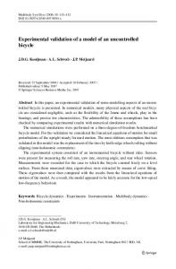
The main components of the equipment can be seen in Fig. 4. In the test arrangement, the source and detector remained stationary, whereas the object rotated on the rotational stage under computer control. The axis of rotation is coincident with the z axis. Repeat scans involving vertical object displacements were achieved by moving the source and detector on precision, computer controlled, vertical linear rails. Details of the experimental equipment and performance capabilities have been reported elsewhere.36 CBCT images of a live rabbit specimen were also acquired using a clinical scanner 共Elekta Synergy, Elekta, Stockholm兲. Table I lists imaging parameters used for each study described here.

Flat Panel Detector

X-Ray Tube Rotation Stage

III.B. Acrylic sphere phantom

FIG. 4. Photograph of test bench used in acquiring projection data. Phantom shown is for illustrative purposes only 共not used in these experiments兲.

important to note that the set of recovered frequency components have been described assuming a continuous source along a circular trajectory 共i.e., using infinite projections兲 and an idealized detector. This situation is not the case in practice, as projections are sampled at a finite number of intervals along the circular trajectory and the detector has finite resolution. However, it is assumed that the sampling in the following experiments is sufficient and will not introduce new artifacts. Conditions for sufficient sampling in terms of projection number and detector pixel sampling have been published.12,36 III. METHODS III.A. Apparatus

An amorphous silicon flat panel detector 共Paxscan 4030A, Varian, Palo Alto, CA兲 with 194 ␮m pixel pitch, and a 600 kHU x-ray tube 共Rad-94, Varian, Palo Alto, CA兲 were used in a CBCT laboratory design for the disk and acrylic sphere experiments described in the following subsections.

In order to identify Cxo in localized regions of space, a phantom was constructed using a set of 3.2 mm diameter acrylic spheres. Spheres were chosen because of their 3D symmetry in the object space and therefore in the frequency domain. This property greatly simplifies the identification of missing frequency components in the Fourier transform. The spheres were housed in polystyrene foam in order to provide a uniform background of near air density, and were aligned at 1 cm intervals. This phantom was positioned vertically such that the first sphere lay on the source plane, whereas the remaining spheres were at increasing z distances. The spheres were imaged coincident with the rotation axis, as well as at an offset, R, in the y direction, in order to observe both the symmetrical and oblique, circular missing cones within the local Fourier space of these subvolumes. Relevant parameters involved in object setup are seen in Fig. 3共a兲. Figure 3共b兲 shows the relationship of maximum and minimum internal angles of the missing cone in frequency space to the real space imaging geometry for an oblique, circular cone. III.C. Missing cone measurements

The theoretical predictions of the size of Cxo were tested using the acrylic sphere data. All images were reconstructed

TABLE I. Imaging and reconstruction parameters. Imaging parameters

Acrylic sphere

Mini-disks

Large disks

Rabbit

Source to axis distance 共cm兲 Source to detector 共cm兲 distance X-ray exposure mode kVp mA ms Filter:

60 96

100 155

100 160

100 154

Pulsed radiographic 100 80 4 4 mm Al+ 0.1 mm Cu 1.125

Pulsed radiographic 120 100 5 2 mm Al+ 0.1 mm Cu 1.125

Pulsed fluoroscopic 120 40 7.5 2 mm Al+ 0.1 mm Cu 1.2

Pulsed radiographic 120 80 10 F1 aluminum bowtie filter 0.55

320 1 121⫻ 121⫻ 121

320 1 125⫻ 125⫻ 125

300 1 120⫻ 120⫻ 120

650 5.5 750⫻ 750⫻ 750

Rotation/projection 共deg.兲 No. of projections Frame rate 共Frames/s兲 Voxel size 共␮m3兲

Medical Physics, Vol. 36, No. 2, February 2009

505

Bartolac et al.: Fourier description and validation of CB artifacts

505

FIG. 5. Surface plots of the function applied to reduce spectral broadening effects in the power spectral density estimation by FFT. The function is applied to avoid sharp discontinuities between the zero padding and the volume edge due to statistical fluctuations.

using the Feldkamp FBP algorithm. Reconstruction subvolumes of 256⫻ 256⫻ 80 voxels were analyzed 共see Table I for voxel size兲, where each subvolume was centered about a single sphere. This dimension was chosen to retain most information in the x and y directions, where the majority of the artifact is expected, simultaneously restricting influence of artifacts from spheres above or below the one examined. Before Fourier transforming the data, a background subtraction was made by subtracting the average polystyrene foam value. Each subvolume was then multiplied by a cylindrical, Hann window function, W共i , j , n兲, such that f win共i, j,n兲 = W共i, j,n兲f r共i, j,n兲 = Wh共i + 1, j + 1兲Wv共n + 1兲f r共i, j,n兲,

共17兲

where f win共i , j , n兲 is the value of the reconstruction volume at index 共i , j , n兲, fr共i , j , n兲 is the value of the original reconstruction volume, Wh共i , j兲 is a circular Hann window degenerate in n, defined as Wh共i + 1, j + 1兲 = i = 0, . . . ,Nh,

冉

冉

共i2 + j2兲1/2 1 1 − cos 2␲ 2 Nh

j = 0, . . . ,Nh,

Nh = 255,

冊冊

, 共18兲

and Wv共n兲 is a linear Hann window degenerate in i and j defined as Wv共n + 1兲 =

冉

冉 冊冊

1 n 1 − cos 2␲ 2 Nv

n = 0, . . . ,Nv

,

Nv = 79.

共19兲

A cylindrical Hann window was preferred over a spherical window in order to better accommodate the shorter z dimension of the subvolume. Surface plots of central vertical and horizontal cross sections of W共i , j , n兲 are seen in Fig. 5. The windowing was performed in order to guarantee a smooth transition to zero mean values at the boundaries of the volume and therefore reduce spectral leakage in the Fourier domain.37 The data were then zero padded to a volume of 256⫻ 256⫻ 256 voxels and transformed using the fast Fourier Transform 共FFT兲. All measurements were made in the Medical Physics, Vol. 36, No. 2, February 2009

Fourier domain, considering only the absolute magnitudes of the frequency components. Working with the magnitude was adequate for identification of the missing frequency components and avoided the necessity of accurate registration of the subvolumes that would be required if the phase components were to be considered. Various methods are possible for verifying the size of Cxo in the experimental data. The chosen method is similar to evaluating an edge spread function at the missing cone boundary. Numerical surface integrals were evaluated over conical surfaces that ranged in size from less than to larger than the expected size of Cxo. The conical integration surfaces had the same oblique angle and orientation as that of Cxo such that at least one surface integral was expected to coincide with its boundary. The result of each integral was normalized with the corresponding result for the sphere that was centered on the source plane. Surface integrals within Cxo would ideally be expected to yield a null value, whereas, values outside it would be expected to have a normalized value of 1 共as frequency components in this region should ideally be the same for all spheres兲. A plot of the integral values as a function of maximum internal angle, ␩2⬘, of the integration surface would be expected to have a maximum derivative at precisely the boundary of the missing cone 共i.e., when ␩2⬘ = ␩2兲. This method was tested using simulated oblique, circular cones of zeros of comparable size created within a volume of ones. The results indicated that the algorithm could accurately return the internal angle of the simulated cones with negligible error. An implicit assumption made in the analysis is that the image of the sphere centered on the source plane will be a “true” reconstruction, whereas images of the spheres above or below the source plane will exhibit a well-defined region of missing frequency components in the Fourier domain. This assumption is compromised by several factors. First, the missing cone is shift-variant and does not have constant size over the volume of a given sphere. However, the spheres were chosen to be small enough to allow for the assumption of shift-invariance to good approximation. Another factor is that the CB artifacts introduced may spread to regions well

506

Bartolac et al.: Fourier description and validation of CB artifacts

z

α

θ

Source Trajectory

FIG. 6. Schematic representation of mini-disk experiment. The z axis corresponds to the axis of rotation. The size of the disks is greatly exaggerated in the illustration for purposes of clarity 共see the text for details兲.

506

the phantom with respect to the kz axis in an obvious way, and allows for a method of probing the frequency response at localized regions of image space. The imaging geometry used in this experiment 共see Table I兲 was chosen to agree with conventional geometries used in IGRT, observing a maximum 共half兲 cone angle of 5.5° 共where a typical range is approximately 5°–7.5°兲. Reconstruction size of the disk phantom was 200⫻ 200⫻ 100 voxels. Background 共foam兲 subtraction and zero padding to equal dimension were performed prior to calculation of the FFTs. III.E. Large disk phantom

beyond the subvolume examined. Although truncation of the artifacts should introduce inaccuracies in the Fourier transform, the impact is expected to be minimal as the majority of the object’s energy is contained within the given subvolume. Further, the effects of spectral leakage that would be introduced by truncating the artifacts are reduced by the window function described previously. Note that the separability of the window function implies separate convolution kernels in the Fourier domain. The effect of these convolutions is expected to have negligible impact to the location of the maximum gradient at the missing cone boundary and is therefore not expected to compromise the analyses presented. Finally, the surface integrals performed excluded regions near the DC component where the boundary of the missing cone is not well defined due to the discrete sampling of the data. III.D. Mini-disk phantom

A mini-disk phantom was constructed using three mylar disks 10.2 mm in diameter, 0.21 mm thick, and spaced by approximately 2.0 mm of polystyrene foam. A schematic representation of the experimental setup illustrating the key parameters involved is seen in Fig. 6. The mini-disk phantom was housed in a polystyrene foam casing and mounted to a rotational microstage, which was used to vary the degree of inclination of the disks, ␪, with respect to the source plane 共see Fig. 6兲. The disks were centered on the rotation axis and imaged at varying distances above the source plane. As the majority of the energy of the disks lies in frequency bands perpendicular to the plane of the disks, changing the parameter ␪ changes the distribution of the frequency spectrum of

kx=0

z

η1

Two distinct large disk phantoms were imaged, one of solid acrylic and the other of cellular polyurethane. The latter material has an internal structure similar to that of trabecular bone. Both disks were 125 mm in diameter, and 1 cm thick. The disk phantoms were imaged parallel and at a displacement of 5 cm above the source plane. The data were analyzed to observe the recovery of internal cellular details at z displacements where planar features with horizontal orientation are expected to be severely distorted. III.F. Rabbit scan

A live, anesthetized rabbit was imaged using a clinical Elekta Synergy unit 共Elekta, Stockholm兲. The rabbit was under free breathing throughout the scan. The dimension of the subvolume chosen for analysis was 64⫻ 64⫻ 64 voxels. This subvolume was chosen to contain soft tissue, bony anatomy, and air. Reconstructions were made using Elekta XVI software. Additional reconstruction parameters are found in Table I. This data were analyzed in order to determine if the missing cone is observable in a more anatomically relevant object under clinical settings. III.G. Exclusion of Other Possible Physical Effects

In order to be convinced that the artifacts seen are due primarily to loss of frequency content and not due to other physical effects, the artifacts should be reproducible by the theoretical removal of local frequency components. Using the mini-disk phantom centered on the source plane as the η2

ky=0

y

FIG. 7. 共a兲 Sagittal view through the center of acrylic sphere imaged at R = 8 cm, z = 7 cm 共windowed兲. 共b兲 Central slice of logarithm of FFT of acrylic sphere in 共a兲 at kx = 0 shows a measurable skew in the null cone as ␩1 is not equal to ␩2. 共c兲 Central slice of logarithm of FFT at ky = 0. Medical Physics, Vol. 36, No. 2, February 2009

507

Bartolac et al.: Fourier description and validation of CB artifacts

(a)

1.0

(b)

507

0.35

Smoothed Derivative Polynomial Fit Residuals (poly) Gaussian Fit Residuals (Gauss) Baseline

0.30

0.8 CSI (normalized)

0.25 o-1

CSI

0.6

dCSI/dη2' ( )

CSI smoothed

0.4

0.20

Gaussian Fit: 2 -4 Reduced χ = 1.6x10 2 Adjusted R = 0.99

0.15 0.10 0.05

0.2

0.00 0.0

0

2

4

6

8

10

12

-0.05

0

2

4

ο

6

8

10

12

ο

η2' ( )

η2' ( )

FIG. 8. 共a兲 Results of surface integrals 共normalized兲 taken over various sized cones as a function of maximum internal angle with respect to the kz axis. 共b兲 Derivative of 共a兲 with corresponding Gaussian and polynomial fits to the peak; peak position should be estimate of ␩2 according to theory.

reference image, and using the assumption of shiftinvariance, the filtering can be carried out in the frequency domain, f filt共x兲 = F−1兵F共k兲 · T共k兲其,

共20兲

where f filt共x兲 is the filtered image, F−1 indicates the inverse Fourier transform, and T共k兲 is a volume of ones with a cone of zeros equivalent to that predicted by theory. This multiplication in the Fourier domain is equivalent to the convolution in the spatial domain of the object function with the theoretical PSF, F−1关T共k兲兴. IV. RESULTS AND ANALYSIS Figure 7共a兲 shows a sagittal view of a sphere reconstructed with an 8 cm offset from the rotation axis, and a height of 7 cm above the source plane. Note that the noise in the image tends to obscure any noticeable artifact. However, sectional views through the logarithm of the 3D FFT, as seen in Figs. 7共b兲 and 7共c兲, show the absence of frequency information within a conical region of space indicating that artifacts are present in the data. Figure 8共a兲 shows a sample plot

(a)

8

of the normalized surface integrals, CSI, as a function of internal angle, ␩2⬘, for the same data set. The shape of the curve is as expected, and increases steadily with increasing ␩2⬘ coming to a maximum value near 1. The solid line represents the data after application of an adjacent mean filter. This filter is expected to provide a smoother first derivative without shifting the location of the peak. Note that the values CSI never approach zero for small ␩2⬘; this characteristic may be partly explained by the presence of noise in the data, partial truncation of the artifacts and spectral leakage not completely eliminated by the window function. A nearestneighbor approximation to the first derivative of the smoothed curve is shown in Fig. 8共b兲. A Gaussian peak function was found to fit this smoothed data adequately with a near unity adjusted R-squared value as well as a small reduced-␹-square value 共displayed on the given plots兲. A third order polynomial was also fit to the peak over a reduced range for additional validation. The location of the peak provides an estimate of ␩2 of the missing cone of frequency components. Angles ␩2 and ␩1 determined using this method are drawn in Fig. 7共b兲. Experimentally determined values of

(b)

7

7

6

6

5

2 1

ο

Gaussian Polynomial Theory Residuals (Gauss) Residuals (Poly)

3

η2 ( )

5

4

ο

η( )

8

4

Gaussian Polynomial Theory Residuals (Gauss) Residuals (Poly)

3 2 1

0

0 2

3

4

5

Z (cm)

6

7

2

3

4

5

6

7

Z (cm)

FIG. 9. 共a兲 Experimentally determined missing cone angle plotted for spheres on the rotation axis 共internal angle= ␩2 = ␩1兲 using Gaussian and polynomial peak fits to derivative data. 共b兲 Experimentally determined ␩2 values for spheres at R = 8 cm. Results show very good agreement with expected values. Medical Physics, Vol. 36, No. 2, February 2009

508

Bartolac et al.: Fourier description and validation of CB artifacts

508 Coronal Views

8.6 cm Sagittal Views 8.6 cm

6 cm

7.4 cm 6.1 cm 4.9 cm 3.6 cm

4 cm

2.5 cm 1.2 cm 0 cm 0o

2 cm

0 cm

2.4o

3.5o

5.1o

6.4o

FIG. 11. Sagittal views of mini-disk phantom imaged at varying heights and degrees of orientation. Increase in angular displacement maintains better resolution of disk edge at increased distance from the source plane. Coronal slices for the case where z = 8.6 cm are also displayed above the sagittal images.

z

FIG. 10. Sagittal slice through acrylic spheres imaged on the rotation axis. Twenty slices were averaged to better illustrate the CB artifacts relative to background noise. Increased artifacts 共shading, streaking兲 are manifested at increasing z distances.

␩2 are also plotted as a function of z for R = 0 and 8 cm in Figs. 9共a兲 and 9共b兲 respectively. Theoretical values are shown as solid lines, and indicate that very good agreement exists between experiment and theory. Figure 10 shows the mean value of 20 slices through the center of the reconstruction on the rotation axis in order to demonstrate the increasing artifact at increased distances z by reducing the influence of noise. Sagittal reconstruction slices of the mini-disk phantom are provided for varying displacements and angular orientations in Fig. 11. Coronal views are also shown for the largest z displacement. Note that in the case of the horizontal disk, the artifacts are symmetric about the rotation axis, and the sagittal view represents any sectional view through the center of the phantom 共i.e., the artifacts extend throughout the axial view兲. In all cases, image recovery of the phantom near the source plane appears well defined, whereas off the source plane the level of artifact evident is varied. Clearly, increasing ␪ resulted in higher fidelity of the disk lamina for regions that are far removed from the source plane. In particular, tilting the disks resulted in less edge distortion, greater fidelity of intensity values and a general reduction of streaking artifacts. Figure 12 demonstrates this result in terms of a frequency domain representation. The missing cone of frequency components predicted by theory is evident for the Medical Physics, Vol. 36, No. 2, February 2009

disk parallel to and above the source plane. Conversely, with greater ␪, the disk maintains more of its frequency content as the majority of its frequency spectrum lies outside the missing cone. Note that artifacts are not completely eliminated by tilting the disk, because the missing cone still affects some portion of its frequency components. This effect is expected as all real finite objects have some frequency content in all directions, and explains the persistence of CB artifacts. Figure 13共a兲 illustrates the process used to reproduce the artifact as indicated by Eq. 共20兲. The frequency components removed were equivalent to that of a cone with a uniform internal angle of 4.9° corresponding to the situation of the mini-disk phantom imaged on the rotation axis and 8.6 cm above the source plane. The same characteristics 共i.e., loss of edge resolution, decreased intensity, streaking兲 are evident between the simulated and experimental data as seen in Fig. 13共b兲. The similarity was verified via the two-dimensional correlation coefficient of central slices, which increased from 0.73 before the convolution step to 0.95 afterwards 共where 1 indicates the same image兲. Five central slices were averaged before calculation of the correlation coefficient in order to reduce the influence of noise in the images. It should be observed that a small, but nonnegligible disagreement can be seen in the intensity values between the simulated and experimental data, as seen in the difference image in Fig. 13共b兲 and the vertical profile of the images in Fig. 13共c兲; this discrepancy may be attributed to the use of a binary discrete filter in the filtering process, which may have introduced a slight over filtration of frequency components. Figure 14 shows the result of imaging disks with differing internal structures on and off the source plane. The acrylic disk is obviously distorted when further from the source plane, characteristic of having high magnitude frequency components on or near the vertical axis; it is worth noting

509

Bartolac et al.: Fourier description and validation of CB artifacts

509 (a)

(a)

z

3D FFT

3D IFFT

×M(k)

(b) Measured Results z=8.6 cm

(b)

Simulated Results z=8.6 cm

Difference Image

(c) 0.16 0.14

exp (z=8.6cm) sim (z=8.6cm) exp-sim (z=8.6cm) exp (z=0cm)

0.12 0.1 0.08 0.06 0.04 0.02 0 -0.02

FIG. 12. Sagittal views of central disk in mini-disk phantom imaged on and above central plane with 共a兲 0° tilt and 共b兲 6.4° of tilt. Sagittal slices of the Fourier transforms are seen to the right. Missing energy is evident in the case where the disk is positioned at 0° and is 8.6 cm off the source plane. By tilting the disk most of its energy now lies out of the range of the missing cone, resulting in a more well defined image. Images are zero padded above and below each disk.

that this effect is very similar to the effect seen in the minidisk phantom but on a larger scale. The cellular structure shows similar blurring, contrast differences and streaking artifacts, but also shows recovery of many internal cellular details under this moderate cone-beam angle 共⬃2.9° 兲. The difference images confirm these observations, showing similar characteristics for both types of disks but also showing good cancellation of internal cellular details in the case of the cellular phantom. Figure 15 shows a central section of the Fourier transform of the subvolume of the rabbit data after windowing with a spherical Hann window. A clear region of decreased energy is observable over a conical region within the Fourier transMedical Physics, Vol. 36, No. 2, February 2009

0

20

40

60

80

100

FIG. 13. 共a兲 Process of artifact simulation by convolution via multiplication in the Fourier domain. The disks imaged on source plane were fast Fourier transformed 共FFT兲 and then multiplied by a function of ones with conical section of zeros resulting in a set of missing frequencies predicted by theory for z = 8.6 cm. The filtered Fourier transform was then inverse Fourier transformed 共IFFT兲 showing the simulated artifact. The resulting disks are compared to the disks imaged experimentally at the same z location in 共b兲 showing clear similarity. The difference image and central profile in 共c兲 show small but nonnegligible intensity differences that may be due in part to slight over filtration of frequency components by use of a binary filter. Images are shown at the same scale.

form. The boundaries of the missing cone that would be expected at the center of the subvolume are overlain on the central section of the FFT for comparison, and indicates fair agreement with observation. Note that nonzero frequency content within the region of the predicted missing cone is expected for a number of reasons. Mainly, the approximation of shift-invariance is poor in this case. In addition, artifacts originating at points near the boundaries of the subvolume are severely truncated, whereas artifacts originating at points outside of the subvolume extend to regions within it, as per Eq. 共16兲. V. DISCUSSION Results from the acrylic sphere experiments agreed well with theoretical predictions, giving strong evidence that CB

510

Bartolac et al.: Fourier description and validation of CB artifacts

(a)

5 cm

0.15

0.1

0 cm 0.05

0

(b)

5 cm

0.15

0.1

0 cm 0.05

0

FIG. 14. 共a兲 Sagittal reconstruction of cellular disk imaged on and off of the source plane. 共b兲 Solid acrylic disk of same dimension as disk in 共a兲 and imaged under equivalent conditions. Difference images between cross sections at different heights are shown below the disk cross sections.

artifacts can be well described by a shift variant cone of missing frequency components in the local Fourier domain. As the missing cone increases in size with distance from the source plane, increased artifact is observed in all reconstructions with increased z distance. However, imaged disks showed better recovery as the angle of inclination with respect to the source plane is increased. This effect can be explained in terms of the placement of signal energy of the disks with respect to the missing cone of frequency components predicted by theory. These results support that the removal of a subset of frequency components will have various effects that depend not only on the imaging geometry, but also on the object being imaged, and in particular the frequency content it presents to the imaging system. From another perspective, as the lines of absent frequency components represent changes in the real object along those directions, it is expected that the resolution of surfaces normal to these directions will be the most degraded. The difference between the effect on planar versus cellular features was illustrated in the images of acrylic and cel-

(a)

(b)

kz ky

y

z x

FIG. 15. 共a兲 Subvolume of rabbit data showing several slices and isosurface of the rabbit spine. 共b兲 Saggital of 3D Fourier transform of volume shown in 共a兲. Volume in 共a兲 is shown prior to use of spherical Hann window. Medical Physics, Vol. 36, No. 2, February 2009

510

lular disks, showing that whereas the boundary of the acrylic disk was lost even at modest cone angles, internal cellular details of the polyurethane disks were apparent at the same imaging location. Using the above-mentioned rationalization, spherical features may appear less degraded in general as the likely affected surfaces are more limited in extent 共namely the upper and bottom-most surfaces兲. This effect aids in explaining why CBCT using a circular trajectory may be in widespread use despite well-documented inability to recover accurate information. It should be clear, however, that although spherical, cellular, or curved features may appear to maintain overall higher fidelity in reconstructions than planar features 共that are near parallel to the source plane兲, CB artifacts will be present in all cases, unless approximations are made, or strong a priori knowledge is present. The cumulative effects of the CB artifacts may be of consequence in terms of introducing contrast reduction, blurring or CT number inaccuracies. These effects are likely of more importance in diagnostic CT than in IGRT, as without a priori knowledge there is greater risk of failing to detect desired features. The results of the cellular disk experiment indicate that a more in depth study of these effects as a function of such factors as object texture is recommended for future study. The methods shown in this paper also showed utility for identifying the presence of CB artifacts in clinical data. In analysis of the rabbit image acquired using a clinical CBCT scanner, no reference 共or “ground truth”兲 data were available for comparison, making it difficult to determine whether CB artifacts were present. Further, even in the presence of accurate reference data, CB artifacts may have very low contrast to noise, or be dominated by other artifacts 共e.g., scatter, beam hardening兲 that obscure noticeable CB artifacts. Analysis of the FFT of a small subvolume, however, confirmed decreased energy in the region of the expected missing cone, indicating that CB artifacts were present. This result suggests that similar analyses may be used to test claims of CB artifact reduction in real data. In addition, the reconstruction fidelity of any localized feature can also be predicted independently of other artifacts using the convolution method posed in this paper if a reference image 共e.g., a CT prior兲 is known. The method can be modified to examine a larger object by piecewise convolution: the larger volume can be divided into sub-volumes, each filtered by a unique transfer function defined by the presented theory and the results added. VI. CONCLUSIONS The results of these experiments support the theoretical predictions of a shift-variant cone of missing frequency components in the Fourier domain when using a circular source and detector geometry in CBCT. This missing cone was successfully identified and measured in the Fourier transform of an acrylic sphere phantom. Recovery of the mini-disk phantom was seen to be strongly dependent on the relative energy distribution of the imaged object with respect to the region of missing frequency components predicted by theory. Image reconstruction of large disk phantoms with varying internal

511

Bartolac et al.: Fourier description and validation of CB artifacts

z

511

P

P

z xo

xo

B

A nS Source Trajectory

FIG. 16. Illustration of the construction of cone A by connecting xo to the circular trajectory using straight lines

structure illustrated the complexity of the observed effect when considering its dependence on the total frequency content of the imaged object. Analysis of the rabbit data indicated that the results are relevant to clinical scanners. ACKNOWLEDGMENTS This work was supported by the National Institute of Health/National Cancer Institute 共R01-CA89081 and R01EB000627兲 and by the H. E. Johns Summer Studentship Program. Its contents are solely the responsibility of the authors and do not necessarily represent the official views of the NIH.

FIG. 18. Illustration of the construction of cone B as a function of normal lines to tangent planes to cone A.

Proof: The vector ␯共␾⬘兲 – po 共Fig. 17兲 defines the aperture of cone A in the source plane, which by definition is circular. Using the law of cosines, the magnitude of this vector can be determined to be 共Fig. 19兲 ps共␾⬘兲 = R cos共␾⬘兲 + 冑␳2 − R2 sin2共␾⬘兲.

共A1兲

Similarly, the aperture of cone B in the source plane is defined by vector n共␾⬘兲 – po, which has magnitude ns共␾⬘兲. From the similar triangles in Fig. 17, ns共␾⬘ + 180兲 is seen to be inversely proportional to ps共␾⬘兲, ns共␾⬘ + 180兲 =

z2o . p s共 ␾ ⬘兲

共A2兲

Using Eqs. 共A1兲 and 共A2兲 the ratio of ns共␾⬘兲 to ps共␾⬘兲 can be formulated as follows:

APPENDIX: PROOF OF THE SHAPE OF THE MISSING CONE As before, xo is considered in the y – z plane at 共0 , R , zo兲 for simplification. Arbitrary xo can be considered by a rotation of coordinates. Consider first, cone A, formed by connecting the source trajectory to xo using straight lines, as shown in Fig. 16. For the sample tangent plane P, a normal line can be constructed containing xo and intersecting the source plane at n, as shown in Fig. 17. Likewise, for each plane tangent to the surface of cone A, a corresponding normal line can be defined. The set of all normal lines constructed in this way forms a distinct cone, B, as shown in Fig. 18. This cone is similar, in the strict mathematical sense, to the missing cone in the Fourier domain. Cone B will be shown here to have a circular aperture in the source plane.

z2o z2 n s共 ␾ ⬘兲 = = o, ps共␾⬘兲 ps共␾⬘ + 180兲ps共␾⬘兲 c

c ⬅ 共 ␳ 2 − R 2兲 ⬎ 0 共A3兲

and is seen to be constant for all ␾⬘. Therefore, the aperture of cone B in the source plane must be circular. As similar cones are defined for arbitrary horizontal plane, the aperture of cone B must be circular in all horizontal planes. The radius of the aperture in the source plane must be half the sum of the maximum and minimum magnitude of ns共␾⬘兲, and can be defined as

xo

φ′

ns (φ′)

ps

νo

α

pS

po nS

n

FIG. 17. Relationship of the normal line to tangent plane P. Medical Physics, Vol. 36, No. 2, February 2009

ps (φ′ + 180)

FIG. 19. Aperture of cones A and B in the plane of the circular trajectory.

512

d=

Bartolac et al.: Fourier description and validation of CB artifacts

冉

冊

tan共␩1兲 + tan共␩2兲 zo , 2

共A4兲

where ␩1 and ␩2 are the minimum and maximum angles of cone B, with respect to the vertical axis, obtained directly from the CB geometry. The axis of cone B, lies in the y – z plane and has angle ␤ to the vertical axis, defined by

␤ = tan−1

冉

冊

tan共␩2兲 − tan共␩1兲 . 2

a兲

共A5兲

Author to whom correspondence should be addressed. Electronic mail: [email protected]; Telephone: 416-946-4501 共x 4049兲; Fax: 416-946-6529. 1 L. A. Feldkamp, L. C. Davis, and J. W. Kress, “Practical cone-beam algorithm,” J. Opt. Soc. Am. A 1, 612–619 共1984兲. 2 H. K. Tuy, “An inversion formula for cone-beam reconstruction,” SIAM J. Appl. Math. 43共3兲, 547–552 共1983兲. 3 D. Finch, “Cone beam reconstruction with sources on a curve,” SIAM J. Appl. Math. 43共4兲, 546–552 共1985兲. 4 P. Grangeat, “Analyse d’un système d’imagerie 3D par reconstruction a partir de radiographies X en géometrie conique,” Ph.D. thesis, École Nationale Supérieure des Télécommunications, Paris, France, 1987. 5 X.-H. Yan and R. M. Leahy, “Derivation and analysis of a filtered backprojection algorithm for cone-beam projection data,” IEEE Trans. Med. Imaging 10共3兲, 462–472 共1991兲. 6 F. Peyrin, R. Goutte, and M. Amiel, “Analysis of a cone beam x-ray tomographic system for different scanning modes,” J. Opt. Soc. Am. A 9共9兲, 1554–1563 共1992兲. 7 A. V. Bronnikov, “Cone-beam reconstruction by backprojection and filtering,” J. Opt. Soc. Am. A Opt. Image Sci. Vis 17共11兲, 1993–2000 共2000兲. 8 K. C. Tam, G. Lauritsch, and K. Sourbelle, “Filtering point spread function in backprojection cone-beam CT and its applications in long object imaging,” Phys. Med. Biol. 47共15兲, 2685–2703 共2002兲. 9 S. Dale and P. Edholm, “Inherent limitations in ectomography,” IEEE Trans. Med. Imaging 7共3兲, 165–172 共1988兲. 10 G. Lauritsch and W. Haerer, “A theoretical framework for filtered backprojection,” Proc. SPIE 3338共1兲, 1127–1137 共1998兲. 11 J. T. Dobbins, III and D. J. Godfrey, “Digital x-ray tomosynthesis: Current state of the art and clinical potential,” Phys. Med. Biol. 48共19兲, R65– 106 共2003兲. 12 J. Brokish and Y. Bresler, “Sampling requirements for circular cone beam tomography,” IEEE Nucl. Sci. Symp. Conf. Rec. 5, 2882–2884 共2006兲. 13 P. Rizo, P. Grangeat, P. Sire, P. Lemasson, and P. Melenec, “Comparison of two three-dimensional x-ray cone-beam-reconstruction algorithms with circular source trajectories,” J. Opt. Soc. Am. A 8共10兲, 1639–1648 共1991兲. 14 H. Hu, “An improved cone-beam reconstruction algorithm for the circular orbit,” Scanning 18共8兲, 572–581 共1996兲. 15 S. W. Lee, G. Cho, and G. Wang, “Artifacts associated with implementation of the Grangeat formula,” Med. Phys. 29共12兲, 2871–2880 共2002兲. 16 H. Yang, M. Li, K. Koizumi, and H. Kudo, “FBP-type cone-beam reconstruction algorithm with Radon space interpolation capabilities for axially truncated data from a circular orbit,” Med. Imaging Technol. 24共3兲, 201– 208 共2006兲. 17 X. Tang, J. Hsieh, A. Hagiwara, R. A. Nilsen, J. B. Thibault, and E.

Medical Physics, Vol. 36, No. 2, February 2009

512

Drapkin, “A three-dimensional weighted cone beam filtered backprojection 共CB-FBP兲 algorithm for image reconstruction in volumetric CT under a circular source trajectory,” Phys. Med. Biol. 50共16兲, 3889–3905 共2005兲. 18 L. Yu, X. Pan, and C. A. Pelizzari, “Image reconstruction with a shiftvariant filtration in circular cone-beam CT,” Int. J. Imaging Syst. Technol. 14共5兲, 213–221 共2004兲. 19 T. M. Benson and J. Gregor, “Three-dimensional focus of attention for iterative cone-beam micro-CT reconstruction,” Phys. Med. Biol. 51共18兲, 4533–4546 共2006兲. 20 K. Zeng, Z. Chen, L. Zhang, and G. Wang, “An error-reduction-based algorithm for cone-beam computed tomography,” Med. Phys. 31共12兲, 3206–3212 共2004兲. 21 S. Valton, P. Berard, J. Riendeau, C. Thibaudeau, R. Lecomte, D. SappeyMarinier, and F. Peyrin, “Comparison of analytical and algebraic 2D tomographic reconstruction approaches for irregularly sampled microCT data,” Conf. Proc. IEEE Eng Med. Biol. Soc. 1, 2916–2919 共2007兲. 22 R. Clackdoyle and F. Noo, “Cone-beam tomography from 12 pinhole vertices,” IEEE Nucl. Sci. Symp. Conf. Rec. 4, 1874–1876 共2001兲. 23 D. A. Jaffray and J. H. Siewerdsen, “Cone-beam computed tomography with a flat-panel imager: Initial performance characterization,” Med. Phys. 27共6兲, 1311–1323 共2000兲. 24 Z. Chen and R. Ning, “Supergridded cone-beam reconstruction and its application to point-spread function calculation,” Appl. Opt. 44共22兲, 4615–4624 共2005兲. 25 A. L. Kwan, J. M. Boone, K. Yang, and S. Y. Huang, “Evaluation of the spatial resolution characteristics of a cone-beam breast CT scanner,” Med. Phys. 34共1兲, 275–281 共2007兲. 26 S. R. Mazin and N. J. Pelc, “A Fourier rebinning algorithm for cone beam CT,” Proc. SPIE 6913, 691323-1–691323-12 共2008兲. 27 J. Hsieh, “A practical cone beam artifact correction algorithm,” IEEE Nucl. Sci. Symp. Conf. Rec. 2, 15/71–15/74 共2000兲. 28 Z. J. Cao and M. W. Tsui, “A fully three-dimensional reconstruction algorithm with the nonstationary filter for improved single-orbit cone beam SPECT,” IEEE Trans. Med. Imaging 40共3兲, 280–288 共1993兲. 29 F. Natterer, The Mathematics of Computerized Tomography 共Wiley, New York, 1986兲. 30 J. Hsieh, Computed Tomography: Principles, Design and Recent Advances 共SPIE, Bellingham, WA, 2003兲, p. 87. 31 B. D. Smith, “Image reconstruction from cone beam projections: Necessary and sufficient conditions and reconstruction methods,” IEEE Trans. Med. Imaging 4, 14–23 共1985兲. 32 A. C. Kak and M. Slaney, Principles of Computerized Tomographic Imaging 共IEEE, New York, 1988兲. 33 S. R. Deans, The Radon Transform and Some of Its Applications 共Wiley, New York, 1983兲. 34 M. Defrise and R. Clack, “A cone-beam reconstruction algorithm using shift-variant filtering and cone-beam backprojection,” IEEE Trans. Med. Imaging 13共1兲, 186–195 共1994兲. 35 H. Kudo and T. Saito, “Derivation and implementation of a cone-beam reconstruction algorithm for nonplanar orbits,” IEEE Trans. Med. Imaging 13共1兲, 196–211 共1994兲. 36 G.-H. Chen, J. H. Siewerdsen, S. Leng, D. Moseley, B. E. Nett, J. Hsieh, D. Jaffray, and C. A. Mistretta, “Guidance for cone-beam CT design: Tradeoff between view sampling rate and completeness of scanning trajectories,” Proc. SPIE 6142, 357–368 共2006兲. 37 F. J. Harris, “On the use of Windows for harmonic analysis with the discrete Fourier transform,” Proc. IEEE 66共1兲, 51–83 共1978兲.