A Locality Preserving Graph Ordering Approach for Implicit Partitioning: Graph-Filling Curves Stefan Schamberger
Jens-Michael Wierum
Fakultät für Elektrotechnik, Informatik und Mathematik
Paderborn Center for Parallel Computing
Universität Paderborn
Universität Paderborn
Fürstenallee 11, D-33102 Paderborn
Fürstenallee 11, D-33102 Paderborn
[email protected]
[email protected]
Abstract Linear orderings defined through space-filling curves are often applied to quickly partition graphs arising in finite element simulations. In applications with constant meshes but a rapidly changing load per element, an ordering has to be determined only once and all subsequent partitionings can be computed very quickly through a simple interval splitting. However, partitionings based on space-filling curves have known drawbacks. Especially when applied to deeply refined meshes or discretizations that contain holes, a high edge-cut is produced. In this paper we present a new linear ordering approach called graph-filling curves. In contrast to space-filling curves, we determine a node ordering based on the graph’s structure rather than on its geometric information. Our experimental evaluation shows that such orderings involving the graphs connectivity information lead to clearly superior implicit partitionings. Keywords: Mesh partitioning, space-filling curves, linear ordering, graph structure
1
INTRODUCTION
Finite elements (FE) are often used to numerically approximate solutions of a partial differential equation (PDE) describing physical processes. The domain on which the PDE has to be solved is discretized into a mesh of finite elements, and the PDE itself is transformed into a set of linear equations defined on these elements [1], which can then be solved by iterative methods such as conjugate gradient (CG). Due to the very large amount of elements needed to obtain an accurate approximation of the original problem, this method became a classical application for parallel computers. The parallelization of numerical simulation algorithms usually follows the single-program multiple-data (SPMD) paradigm: Each processor executes the same code on a different part of the data. This means that the mesh has to be split into P sub-domains (where P is the number of processors) and each sub-domain is then assigned to one of the processors. Since iterative solution algorithms mainly perform local operations, i. e. data dependencies are
defined by the mesh, the parallel algorithm requires communication only at the partition boundaries. Hence, the efficiency depends on two factors: An equal distribution of the data (work load) on the processors and a small communication overhead achieved by minimizing the number of edges between different partitions. Since the graph partitioning problem only represents a subproblem of the overall FE computation, it has to be solved fast and as space-efficient as possible. Due to the size of the involved meshes, state-of-the-art graph partitioning libraries like Metis [2], Jostle [3], Chaco [4], or Party [5] usually follow the multilevel scheme. Vertices of the graph are contracted and a new level consisting of a smaller graph with a similar structure is generated. This is repeated, until in the lowest level only a small graph, sometimes only with 2 vertices, remains. The partitioning problem is then solved for this small graph and vertices in higher levels are assigned to partitions according to their representatives in lower levels. Then a local refinement phase is applied to further enhance the current solution. In most cases, the local refinement process is based on the Fiduccia-Mattheyses method [6], a run-time optimized version of the Kerninghan-Lin (KL) heuristic [7]. This process finally leads to a high-quality partitioning of the original graph in a reasonable short time. However, in some applications the node weights representing the finite elements’ computational load change rapidly and unpredictably. Also if the number of available processors changes frequently, many repartitions of the same graph are needed. In these cases, the load has to be rebalanced very quickly to avoid the overall runtime being dominated by the load-balancing algorithm. An extremely fast approach to balance meshes containing nodes with highly fluctual computational load is given by implicit partitioning: Initially, the mesh’s nodes are rearranged according to a certain scheme, such that the following partitioning problems are reduced to simply splitting the node list into intervals of appropriate size. To keep the edge-cut reasonable low and the partitions compact, the node ordering has to preserve locality.
post.peano.grid16.ps 29.04.02 10:49
size 256 (-1-1073782286)
Hilbert
post.lebesgue.grid16.ps 29.04.02 11:39
Lebesgue
size 256 (-1-1073782286)
post.sierpinski.grid16.ps 04.09.02 10:04
size 256 (-1-1)
Sierpi´nski
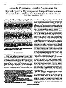
Figure 1. Space-filling curve structures in the 16 × 16 grid.
A popular method determining such an arrangement are space-filling curves. Space-filling curves are geometric representations of bijective mappings M : {1, . . . , N m } → {1, . . . , N}m . The curve M traverses all N m cells in the mdimensional grid of size N. They have been introduced by Peano and Hilbert in the late 19th century. An (historic) overview on space-filling curves is given in [8]. The curves used in the experimental part of this paper are plotted in figure 1. In [9], it is shown that partitionings based on connected space-filling curves are “quasi optimal” for regular grids and special types of adaptively refined grids. In these cases, the edge-cut is bounded by C · (|V |/P)(d−1)/d , where |V | denotes the number of vertices, P the number of partitions, and d the dimension of the graph. The constant C depends on the curve type and has been determined for some of them on 2-dimensional regular grids in [10]. Comparisons between advanced graph partitioning heuristics and space-filling curves have been undertaken and results are presented for example in [11, 12, 13]. They reveal that the advanced partitioning tools determine solutions with a lower edge-cut. Especially in some configurations that often occur in FE mesh partitioning, space-filling curves tend to produce partitionings of bad quality. The most important cases are: The number of requested partitions is small, the mesh contains holes, or unevenly refined regions exist whose expansion is of lower dimension than the overall problem (e. g. a 2-dimensional area within a 3dimensional FE mesh). This is a consequence of ignoring the provided connectivity information but only relying on nodal coordinates. Finding a linear ordering of a graph is a combinatorial problem and has been studied extensively with respect to various objective functions. There exists a number of theoretical bounds, approximation algorithms, and heuristics. A good overview and many references to related topics can be found in [14]. Most of the metrics considered are not suited to determine good orderings for implicit graph partitioning. Even the wire-length metrics (also denoted as edge sum, minimum 1-sum, or bandwidth sum) that does reflect some kind of locality, does usually not lead to a small global edge-cut of the implicit partitionings. For example, optimizing this metrics always results in placements of the first and last vertex of the curve far away of each other, what is not required and usually not helpful.
A metrics very similar to the wire-length is considered in [15]. There, the authors address the problem of extending a curve in a triangular mesh after a refinement step. They prove the existence of so called self-avoiding walks and present a linear time algorithm to find these. Another approach based on refinement tree traversals has been presented in [16]. In this paper we present a new ordering method that is based on structural information of the mesh. Arranging the nodes according to such an ordering, the quality of the implicit determined partitionings can be improved significantly compared to space-filling curve based solutions. The remainder of this paper is organized as follows. In the next section, we present the main idea of the new ordering algorithm. We describe the necessary ingredients for our approach and present a greedy implementation. The results we obtain with it are presented in section 3 and are compared with those of the graph partitioning package Metis and space-filling curve based solutions. Finally, we conclude and refer to further research directions.
2
GRAPH-FILLING CURVES
In this section we present a new linear ordering approach well suited for implicit partitioning. We describe the drawbacks of space-filling curves, the general improvement idea, and present an experimental implementation.
2.1
The Main Idea
Space-filling curves (SFC) are continuous curves which completely fill up higher dimensional spaces such as squares or cubes. Due to their fractal nature, they possess locality preserving properties with respect to different metrics. Hence, the area covered by an arbitrary interval of such a curve has a limited surface, which differs at most by a constant factor from the optimal volume–surface relation [9, 10]. This property can be exploited to partition a graph, because each partition should have a limited surface, i. e. a small number of outgoing edges as well. Although space-filling curves were initially defined on grids, they can also be used to determine node orderings in unstructured meshes. The graphs’ vertices are separated recursively and aligned according to the underlying curve structure. The recursion is repeated until each subpart contains a single vertex. From the definition of the curves follows that the corresponding separators are n − 1dimensional hyper-planes in the n-dimensional space. The locality preserving properties ensure that each interval of the curve forms a partition with a to some extend limited number of edges to the remainder of the graph [13]. However, this only holds as long as the given mesh structure allows a suitable embedding of the curve, like it is the case for regular grids. If this is not possible, the purely geometric separation destroys the locality properties of the ordering which are necessary to find good graph partitioning solutions. Especially if the graph contains steeply refined
Figure 2. Defining a locality preserving curve is often difficult if the graph separation is based on geometric information (left). A separation based on graph partitioning can overcome this problem (right).
regions and holes, a space-filling curve only based on geometric information will no longer preserve locality. An example is given in figure 2 sketching a graph with two holes in a refined area. On the left picture the graph is separated according to the first level of a SFC ordering. Here, large parts of the cuts traverse steeply refined areas. Since boundaries of partitions based on orderings often coincide with the separators of high levels, the resulting implicit partitioning quality can be expected to be quite poor. Furthermore, a curve has to cover every vertex in a region before entering the next one. Hence, in the shown case, the curve loses much of its locality. In contrast, the separators displayed in the right picture are based on a high quality 4-partitioning. Assuming that these separators are part of the resulting partitioning, it becomes clear that a solution with a much lower edge-cut can be found. The question arises if there exists a more suitable method to subdivide the vertices and arrange them in a locality preserving way than it is possible with SFCs. One possible approach is presented in this paper. Its main idea is to construct a curve which omits the use of geometry based separators and static ordering rules that can hardly be embedded into unstructured meshes.
2.2
The Algorithm
To find a suitable linear locality preserving ordering, we propose the following two-phase algorithm. In the first phase, the graph is recursively partitioned and the corresponding hierarchy tree is constructed. In the second phase, an appropriate rearrangement within the tree is performed, which is supposed to improve the locality of the ordering. In the partitioning phase, each recursion divides the current subgraph into k parts, where k is a small constant. This phase continues until only one vertex in each subgraph remains. The first two levels of this process are illustrated in figure 3 for k = 3. Traversing the constructed hierarchy defines the order of its leaf nodes representing the graph’s vertices. The second phase of the algorithm tries to optimize this ordering by suitably rearranging the successors of each node in the tree. This means that we allow a locally restricted reordering of nodes on the same level. Since our aim is to determine orderings that induce a small global edge-cut, we propose to link partitions with a
Figure 3. Phase 1: The construction of a hierarchy based on a partitioning algorithm. In every level, the (sub-)graph is divided into 3 parts (left). The resulting tree hierarchy is shown (right).
large common boundary. This increases the probability that the curve will still be connected in the lower levels of the tree’s hierarchy. A possible rearrangement in the hierarchy tree is sketched in figure 4. Starting with the solution given in figure 3, the nodes representing subgraphs G2 and G3 are exchanged, as well as the nodes G3.1 and G3.3 . The nodes G2.i are shifted to the right, respectively. Note, that all rearrangement operations involve nodes with the same successor only. Hence, the previously defined orderings in higher levels remain unchanged. On the right hand side of the figure, the old (top) and the new (bottom) curve is plotted in the sketched graph. From the description of the algorithm follows that there is an obvious dependency between the choice of the parameter k and the number of possible rearrangements in the second phase. A small k leads to a high grade of convolution while a large k increases the flexibility in the reordering of the hierarchy. In the case of bisections (k = 2), there are obviously only two possibilities to traverse the successors of each node. Due to the relationship to the graph’s structure rather than to its geometric shape we call the traversals generated by recursive or iterative partitioning graph-filling curves (GFC).
2.3
Implementation Details
As we have seen in our experiments, high level separators have a large influence on the final induced implicit partitionings. Hence, it is self-evident to realize them through partition boundaries determined by sophisticated graph partitioning heuristics. In our experimental implementation of the GFC-algorithm we apply the Party library. By choosing a graph partitioning library to determine the vertex sets in each level, we try to keep as many as possible edges inside one part and therefore enlarge the locality of the resulting curve. In our experiments, we tested different granularities in the partitioning phase, ranging from 2- to 7-partitionings. Here, results for k = 3 and k = 4 are presented. For the second phase, we have implemented a greedy
airfoil1.sfc.ps 02.04.04 14:09
Figure 4. Phase 2: Traversing the hierarchy defines a curve. Its locality might be improved by exchanging subgraphs (and their successors) of the same levels.
algorithm following a top down strategy in the hierarchy tree. Our objective is to maximize the connectivity of partitions along the curve in each level. At first, the successors of the root are ordered such that the sum of the edge-cuts between neighboring partitions is maximized. An analogue strategy is applied to all nodes of the hierarchy tree. Furthermore, inner nodes use additional information of their right neighbor. To rate a possible arrangement, the sum of local edge-cuts is increased by the maximum edge-cut of the rightmost successor’s partition to the best fitting successor of the right neighbor node. Applying this to the example given in figure 4, we proceed as follows. When examining node G1 , the weight of the supposed order G1.1 , G1.2 , G1.3 is increased by the number of shared edges between G1.3 and G3.3 . This extension increases the connectivity of the generated curve. For the right neighbor (in this case G3 ), we have two possibilities to achieve a high connectivity in this level: (a) Start with the proposed partition G3.3 and find the order of (G3.1 , G3.2 ) followed by any G2.i with the highest weight; (b) Search the best order in (G3.1 , G3.2 , G3.3 ) followed by any G2.i . If the weight of case (a) increased by the benefit of including the cut between G1.3 and G3.3 is higher than the weight of case (b), the curve is constructed according to (a), otherwise it follows (b). This algorithm only performs properly as long as a node of the hierarchy tree represents several vertices of the graph. A special local phase, which smoothes the curve on the last tree level is missing up to now. However, the effect of this lack is limited and is discussed in conjunction with our experimental evaluation.
3
EVALUATION
In this section we examine the locality preserving properties of the new ordering approach. The considered metrics is the classical edge-cut since it models the data interdependencies and is therefore proportional to the communication volume. We compare the partition quality of orderings derived from GFC and SFC. However, since the k-partitioning problem of arbitrary graphs is NP-hard, the optimal results for graphs of reasonable size are not known. Hence, we set the achieved qualities in relation to the re-
size 4253
SFC
airfoil1.sfc.ps 02.04.04 14:06
size 4253
GFC
Figure 5. Benchmark airfoil1: Comparison of SFC (left) and GFC (right) based implicit 5-partitionings.
sults obtained by Metis, a widely applied graph partitioning library.
3.1
An Example: Ordering airfoil1
To provide a detailed example, we first analyze the space-filling and graph-filling curves on the small airfoil1 graph. This unstructured mesh consists of 4 253 vertices and 12 289 edges and contains holes with a fine discretized region around them. Figure 5 shows the computed orderings indicated by a curve of decreasing saturation and the resulting 5-partitionings in case of a SFC (left) and a GFC (right). For the SFC approach we applied the Hilbert curve while the GFC is based on recursive bi-partitioning combined with the proposed ordering algorithm presented in section 2. The SFC ordering starts in the lower left corner and follows the Hilbert curve to the lower right corner. The course of the separators of the higher levels is well visible, especially the first vertical one which results in only one connection between the left and the right part of the curve. As one can see, there are a lot of curve segments crossing the holes in the graph. Partitions based on such an ordering will contain vertices from both sides of the hole as demonstrated below for the implicit 5-partitioning. As expected, the upper left partition contains vertices from above as well as from below the large hole. Furthermore, the course of the horizontal separator of the highest level leads to a very large cut between both partitions on the left hand side. A more detailed view reveals similar bad cuts between other
3.2
The Test-Set: Evaluated Meshes
For the remaining experiments, we used a set of well known 2- and 3-dimensional FEM graphs. Many of them have been used to compare various graph partitioning libraries and are available over the Internet. Table 1 gives an overview of the test set and some of the graphs’ properties. The 2-dimensional graphs biplane.9 and shock.9 have a grid-like structure in which all edges are axis aligned. crack and big are much more unstructured with arbitrarily oriented edges at triangular elements. All of the 3dimensional benchmarks are discretized by tetrahedrons. Especially rotor has a widespread zone consisting of a very fine discretization.
Table 1. The characteristics of the evaluated graphs.
graph crack big biplane.9 shock.9 brack rotor wave hermes
|V | 10 240 15 606 21 701 36 476 62 631 99 617 156 317 320 194
|E| 30 380 45 878 42 038 71 290 366 559 662 431 1 059 331 3 722 641
degavg 5.93 5.88 3.87 3.91 11.71 13.30 13.55 23.25
dim 2 2 2 2 3 3 3 3
3
edge-cut relative to Metis
partition pairs. The GFC ordering starts close to the right end of the large hole in the area of fine discretization. The curve continues below the smallest and the left hole. It surrounds the group of holes in counter clockwise order and ends close to its starting point. On a first view, the curve seems quite convoluted. This effect emerges from a missing local optimization phase. A closer look reveals that these obvious misalignments of the curve almost always affect only vertices close together. Hence, it only influences the quality of an induced partition at its entrance into the partition and its exit from it. Furthermore, one can see that the curve crosses the holes only once. The resulting 5-partitioning is shown in the lower right illustration. Apart from some single vertices, only one partition is disconnected and split into two parts. The partition in the lower left corner has additional vertices in the region between the two smaller holes. With a global edge-cut of 318, the implicit 5partitioning based on the GFC approach is much better than the one obtained according to the Hilbert curve, which has an edge-cut of 624. As a comparison, elaborated graph partitioning heuristics like Party and Metis are able to find separators with an edge-cut of 202 and 231, respectively. Although the latter values are still smaller, these numbers give an indication of the improvement due to the new linear ordering approach. The following, more comprehensive evaluations show that the new structure based ordering approach produces partitionings with a quality much closer to the best known solutions than its geometric counterparts.
SFCS GFC3 GFC4
2.5
2
1.5
1
0.5
2
4
8 16 32 number of partitions
64
128
Figure 6. Benchmark big: SFC vs. GFC ordering.
3.3
Results
In figure 6, the edge-cut of the implicitly generated partitionings based on SFC and GFC orderings in the mesh big is displayed. As in all following experiments, the number of created partitions ranges from 2 to 128. To be able to estimate the benefit of GFC as well as the overall quality, the obtained edge-cuts are normalized to those calculated by Metis. Note, that in this case the SFC ordering is based on the Sierpi´nski curve, since further examinations have revealed that this ordering leads to the best solutions in unstructured meshes. The GFC ordering depends on the parameter k for the recursive partitioning in phase 1. The results for k = 3 and k = 4 are labeled as GFC3 and GFC4 , respectively. It becomes obvious that the GFC approach is superior to SFC over the whole range of examined partition numbers. Remarkable is the fact that in contrast to SFC, the partition quality induced by the GFC ordering is less influenced by the number of desired partitions. Most of the solutions have a quality better than 1.5 relative to Metis. That means that the obtained implicit partitioning has an increase in edge cut of less than 50% compared to the elaborated graph partitioning library. Values lower than 1 arise from the good solutions delivered by the Party library, which we apply as the underlying graph partitioner. The GFC profits directly from these separators which are better than those of Metis. As mentioned above, the quality of resulting partitionings depends on the right choice of k. Especially for a small number of partitions, the edge-cut of the obtained results befalls a high variation. For example, the GFC4 ordering leads to good results in case of 2- and 4-partitionings but is bad in case of the 3-partitioning. In this case GFC3 performs much better. Although this behavior has been expected, it is interesting to see that the difference almost disappears for larger number of partitions. Further experiments with other small values of k have confirmed this observation. Figure 7 shows the results for the 3-dimensional FE
6
4 3 2 1 0
SFCH GFC3 GFC4
1.6 edge-cut relative to Metis
5 edge-cut relative to Metis
1.8
SFCH SFCL GFC3 GFC4
1.4 1.2 1 0.8
2
4
8 16 32 number of partitions
64
0.6
128
2
4
8 16 32 number of partitions
64
128
Figure 7. Benchmark rotor: SFC vs. GFC ordering.
Figure 8. Benchmark grid: SFC vs. GFC ordering.
mesh rotor. Again, the presented values are normalized according to the results obtained by Metis. The SFC ordering is based on the 3-dimensional variants of the Hilbert and the Lebesgue curve described in [13], labeled by SFCH and SFCL , respectively. Most of the values obtained for both SFC variants lie in the range of 3 to 4. The Hilbert curve induces even worse results in case of small partition numbers with a peak (8.7) in case of the bisection. Note that this value is omitted to allow a more concise scaling. For partitionings into 5 or less parts the Lebesgue curve reaches better qualities, but the overall behavior of both geometric schemes is not acceptable for most applications. The quality of partitions induced by GFC with parameters k = 3 and k = 4 are much closer to the results of Metis. 79% (k = 3) and 84% (k = 4) of the achieved edge-cuts are below the factor 1.4. The averages in normalized quality are 1.33 (k = 3) and 1.30 (k = 4). This means that we can expect an increase in edge-cut of just one third compared to Metis, instead of a factor of 3 to 4. The variation of the values is much smaller compared to SFC orderings and again less dependent on the number of partitions. Furthermore, different values for the parameter k have less influence while the choice of the space-filling curve type (Lebesgue vs. Hilbert) has dramatic consequences on the partition quality, especially for a small number of parts. The experimental results for all graphs of our test-set listed in table 1 are summarized in table 2. The edgecuts achieved by Metis, SFC, and GFC are given for the 4-, 16-, and 64-partitioning. For the unstructured meshes crack and big, the ordering was generated according to the structure of the Sierpi´nski curve, while all others follow the Lebesgue curve or its 3-dimensional extension. Among the traditional SFC orderings, these settings achieve the best or close to the best results. The GFC approach is based on the parameter k = 3 for the recursive partitioning because k = 2 or k = 4 will automatically induce high quality Ppartitionings if P is a power of 4. Table 2 shows that in almost all cases GFC outperforms
SFC, in many cases even dramatically. Only in two settings (64-partitioning of crack; 16-partitioning of shock.9) the edge-cut of the partitioning induced by a SFC ordering is slightly better than the one of the solution based on GFC. Compared to Metis, the edge-cut of solutions computed with SFC is in average about 2.1 times as high ([1.35, . . . , 3.82]). Applying GFC instead, this factor can be decreased down to a value of 1.4 ([1.26, . . . , 1.86]). Note, that the computation time of the GFC algorithm is longest. This is due to the multiple invocation of the graph partitioner as well as the additional rearrangement phase. However, the ordering for a graph has to be determined only once and all implicit partitionings can thereafter be constructed in almost no time. Hence, most of the computation time can be shifted into the initial mesh generation process.
3.4
Edge Cut in Regular Grids
In regular grids all space-filling curves with orthogonal separators produce orderings of similar locality [13] close to the optimum with respect to their partitioning capabilities. Hence, it is useful to compare the partitioning quality of SFC and GFC also for this graph type. Results for the Hilbert-curve and the GFCs based on 3- and 4-partitioning the 100 × 100 grid are shown in figure 8. Up to 16-partitionings, both approaches result in a comparable edge-cut, especially when comparing the GFC based on 4-partitioning. For finer partitionings the SFC ordering performs better, with an relative edge cut of 1.2 for more than 100 partitions compared to 1.4 of the GFC method. A closer look at the total edge-cut shows that the average number of outgoing edges per partition is about 40 for Metis, 48 for SFC-, and 56 for GFC-ordering. More than half of the gap is caused by unnecessarily long partition boundaries. This reveals that a final phase smoothing the curve is missing in our implementation. With such an additional optimization, the number of outgoing edges could be reduced by about 2 to 4, both at the entrance of the curve into the partition and at its exit.
Table 2. Comparison of edge-cuts: Metis, SFC, and GFC.
graph crack big biplane.9 shock.9 brack rotor wave hermes_all
4
Metis 408 344 193 449 3 493 8 829 21 682 46 258
4-partitioning SFC GFC 1 066 648 993 481 468 256 637 632 7 696 6 508 27 976 12 726 32 101 27 349 121 152 65 364
16-partitioning Metis SFC GFC 1 218 2 013 1 831 1 099 2 267 1 701 800 1 235 1 086 1 208 1 675 1 700 13 225 28 086 18 696 24 477 93 526 32 996 48 183 78 592 65 050 119 219 266 479 154 419
CONCLUSION AND FUTURE WORK
In this paper we have presented a new approach to determine linear orderings of graphs, called graph-filling curves. These are more suitable for implicit partitioning on unstructured meshes than those based on space-filling curves. Related to the graph’s structure rather than its geometric information, the new orderings significantly reduce the resulting edge-cut. A relative comparison with elaborated graph partitioning heuristics like Metis shows that the loss of quality is lower than in case of the geometric approaches and basically independent of the partition number. We think that the presented approach opens a wide field of further research. For example, the proposed concept does not depend on fully balanced partitions like they are currently implemented in the first phase of our algorithm. Increasing the imbalance allowance of the partitioner, the (sub-)graphs could be created with less edge-cuts what possibly increases the locality of the curve and therefore the induced partition quality. Additionally, it might be helpful to handle the granularity of partitioning in this phase more flexible. Furthermore, the present implementation of the second phase is obviously preliminary. Although it is able to determine curves with high locality, this phase might contain the greatest opportunities for further improvements. The greedy algorithm working top down and “left to right” through the hierarchy is too rigid to find the best results within this new concept. The development of a more elaborated heuristic for the second phase could benefit from the definition of a metrics describing the necessary locality properties for implicit partitioning. The common metrics for linear graph layouts are not suited for this task. Finally, there is the need for a smoothing function at the end of the ordering mentioned in sections 2 and 3.
REFERENCES [1] G. Fox, R. Williams, and P. Messina, Parallel Computing Works!. Morgan Kaufmann, 1994. [2] G. Karypis and V. Kumar, “A fast and high quality multilevel scheme for partitioning irregular graphs,” SIAM Journal on Scientific Computing, vol. 20, no. 1, pp. 359–392, 1998.
64-partitioning Metis SFC GFC 2 781 3 927 3 944 2 843 4 854 4 166 1 906 2 888 2 653 2 902 3 915 3 832 29 432 61 054 39 755 52 190 182 657 67 499 94 342 138 787 120 314 241 771 473 081 322 317
[3] C. Walshaw and M. Cross, “Parallel optimisation algorithms for multilevel mesh partitioning,” Parallel Computing, vol. 26, no. 12, pp. 1635–1660, 2000. [4] B. Hendrickson and R. Leland, “A multi-level algorithm for partitioning graphs,” in Supercomputing, 1995. [5] S. Schamberger, “Improvements to the helpful-set heuristic and a new evaluation scheme for graphs-partitioners,” in International Conference on Computational Science and its Applications, LNCS 2667, pp. 49–59, 2003. [6] C. M. Fiduccia and R. M. Mattheyses, “A linear time heuristic for improving network partitions,” in Design Automation Conference, 1984. [7] B. W. Kernighan and S. Lin, “An efficient heuristic procedure for partitioning graphs,” The Bell System Technical Journal, vol. 49, no. 2, pp. 291–307, 1970. [8] H. Sagan, Space Filling Curves. Springer, 1994. [9] G. Zumbusch, Parallel Multilevel Methods: Adaptive Mesh Refinement and Loadbalancing. Teubner, 2003. [10] J. Hungershöfer and J.-M. Wierum, “On the quality of partitions based on space-filling curves,” in International Conference on Computational Science, LNCS 2331, pp. 36–45, 2002. [11] B. Hendrickson and K. Devine, “Dynamic load balancing in computational mechanics,” Computer Methods in Applied Mechanics and Engineering, vol. 184, pp. 485–500, 2000. [12] K. Schloegel, G. Karypis, and V. Kumar, “Graph partitioning for high performance scientific simulations,” in The Sourcebook of Parallel Computing. Morgan Kaufmann, 2002. [13] S. Schamberger and J. M. Wierum, “Graph partitioning in scientific simulations: Multilevel schemes vs. space-filling curves,” in Parallel Computing Technologies, LNCS 2763, pp. 165–179, 2003. [14] J. Diaz, J. Petit, and M. Serna, “A survey of graph layout problems,” ACM Comput. Surv., vol. 34, no. 3, pp. 313–356, 2002. [15] G. Heber, R. Biswas, and G. R. Gao, “Self-avoiding walks over adaptive unstructured grids,” Concurrency: Practice and Experience, vol. 12, no. 2-3, pp. 85–109, 2000. [16] W. F. Mitchell, “The Refinement-Tree Partition for Parallel Solution of Partial Differential Equations,” J. Res. Natl. Inst. Stand. Technol., vol. 103, no. 4, pp. 405–414, 1998.