IEEE JOURNAL OF SELECTED TOPICS IN APPLIED EARTH OBSERVATIONS AND REMOTE SENSING, VOL. 6, NO. 3, JUNE 2013
1688
Locality Preserving Genetic Algorithms for Spatial-Spectral Hyperspectral Image Classification Minshan Cui, Student Member, IEEE, Saurabh Prasad, Member, IEEE, Wei Li, Student Member, IEEE, and Lori M. Bruce, Senior Member, IEEE
Abstract—Recent developments in remote sensing technologies have made hyperspectral imagery (HSI) readily available to detect and classify objects on the earth using pattern recognition techniques. Hyperspectral signatures are composed of densely sampled reflectance values over a wide range of the spectrum. Although most of the traditional approaches for HSI analysis entail per-pixel spectral classification, spatial-spectral exploitation of HSI has the potential to further improve the classification performance—particularly when there is unique class-specific textural information in the scene. Since the dimensionality of such remotely sensed imagery is often very large, especially in spatial-spectral feature domain, a large amount of training data is required to accurately model the classifier. In this paper, we propose a robust dimensionality reduction approach that effectively addresses this problem for hyperspectral imagery (HSI) analysis using spectral and spatial features. In particular, we propose a new dimensionality reduction algorithm, GA-LFDA where a Genetic Algorithm (GA) based feature selection and Local-Fisher’s Discriminant Analysis (LFDA) based feature projection are performed in a raw spectral-spatial feature space for effective dimensionality reduction. This is followed by a parametric Gaussian mixture model classifier. Classification results with experimental data show that our proposed method outperforms traditional dimensionality reduction and classification algorithms in challenging small training sample size and mixed pixel conditions. Index Terms—Gaussian mixture model, genetic algorithm, hyperspectral imagery, local Fisher’s ratio.
I. INTRODUCTION
R
ECENT developments in remote sensing technologies have made hyperspectral imagery (HSI) readily available to detect and classify objects on the earth using pattern recognition techniques. Hyperspectral signatures are composed of densely sampled reflectance values over a wide range of the electro-magnetic spectrum. Although most of the traditional approaches for HSI analysis entail per-pixel spectral classification, spatial-spectral exploitation of HSI has the potential to further improve the classification performance—particularly when there is unique class-specific textual information in the Manuscript received October 11, 2012; revised February 19, 2013 and April 05, 2013; accepted April 06, 2013. Date of publication May 15, 2013; date of current version June 17, 2013. This work was supported in part by the National Aeronautics and Space Administration under Grant NNX12AL49G, and by the University of Houston, College of Engineering Startup Funds. M. Cui and S. Prasad are with the Electrical and Computer Engineering Department, University of Houston, Houston, TX 77004 USA (corresponding author e-mail:
[email protected]). W. Li is with the University of California, Davis, CA 95616 USA. L. M. Bruce is with Mississippi State University, Starkville, MS 39762 USA. Color versions of one or more of the figures in this paper are available online at http://ieeexplore.ieee.org. Digital Object Identifier 10.1109/JSTARS.2013.2257696
scene. In recent work, incorporating spatial context [1]–[3] into per-pixel spectral classification has shown to substantially improve classification performance for HSI. One open challenge with deriving spatial features from HSI is the further deterioration in the over-dimensionality problem—by deriving spatial information from each spectral band, the dimensionality of the feature space is expected to increase substantially, and many of the features derived are likely to be redundant. A common approach to address the problem of over-dimensionality and small-sample-size is dimensionality reduction. There are two general approaches for dimensionality reduction—selection-based and projection-based. The purpose of feature selection is to find a subset of all available features without a projection based on some criterion function. Most importantly, the subset of selected features should not significantly degrade the performance of the classifier. Sequential Feature Selection (SFS) [4], [5] is a traditional feature selection method that selects the pertinent subset of features. It typically involves two steps: forward sequential selection and backward sequential rejection. The main disadvantage of SFS is that it is unable to reevaluate features that have been added or removed. Since Genetic Algorithms (GA) are well known to efficiently solve combinatorial optimization problems, GA is an attractive alternate to heuristic based searching algorithms. Unlike SFS, GA is able to potentially reevaluate all of the features at each iteration. In previous work, GA has been shown to work very well for a variety of feature selection tasks [6]–[9]. Projection based dimensionality reduction is an alternate way to address the over-dimensionality problem. It is a technique that projects raw features into a lower dimensional subspace. There are many feature projection techniques have been proposed in literature such as Principal Components Analysis (PCA), Linear Discriminant Analysis (LDA) [10], Regularized LDA (RLDA) [11], [12] and Local Fisher Discriminant Analysis (LFDA) [13] etc. The primary disadvantage of these methods is that often, algorithms such as LFDA and LDA necessitate a reasonably large training sample size to effectively learn the projection. This paper proposes a hybrid dimensionality reduction method called GA-LFDA where GA based feature selection and LFDA based feature projection are performed in a raw spectral-spatial feature space. The goal of GA-LFDA is to alleviate the problem of over-dimensionality and small sample size problems, particularly when dealing with very high dimensional feature spaces such as those comprised of feature-level fusion of spectral and spatial information from an HSI cube.
1939-1404/$31.00 © 2013 IEEE
CUI et al.: LOCALITY PRESERVING GENETIC ALGORITHMS FOR SPATIAL-SPECTRAL HYPERSPECTRAL IMAGE CLASSIFICATION
1689
TABLE I SIX COMMON FEATURES USED IN GLCM
Fig. 1. (a) Intensity values of an image and (b) corresponding counts matrix of the image defined by a position operator as “upper right”.
The rest of the paper is organized as follows. In Section II, we briefly introduce the proposed spatial feature extraction for HSI classification. In Section III, conventional dimensionality reduction methods are described. The proposed GA-LFDA algorithm is presented in Section IV. In Section V, we provide a description of two popular parametric classifiers that are used in this work. The experimental setup and results are presented in Section VI. Finally, we provide concluding remarks in Section VII. II. SPATIAL FEATURE EXTRACTION FOR HSI CLASSIFICATION Conventional HSI classification is typically based on exploiting per-pixel spectral content, often ignoring the structure of the spatial features in the image. In recent work, several researchers have investigated different techniques to incorporate spatial contextual information into the classification task [6]–[9] and have shown that such approaches yield improved classification compared to the per-pixel spectral reflectance only classification. In this work, we develop a novel approach to fully exploit the spatial content of the HSI via using Grey Level Co-occurrence Matrix (GLCM) derived textural features extracted from each spectral channel. GLCM spatial measurements have been a popular method for spatial feature extraction in remotely sensed images since they were first introduced by Haralick in the 1970s [14]. The GLCM describes spatial context of images based on how frequently two grey levels appear according to a position operator within an image. For a position operator determining relative position between two grey levels, we can define a matrix that counts the number of times a pixel with grey-level occurs at position from a pixel with grey-level . Fig. 1 shows an image that has three different grey-levels denoted by different colors and its corresponding counts matrix defined by the position operator as “upper right”. If we normalize the counts matrix by the total number of pixels and make it symmetrical by adding the , we get a GLCM, . transposed counts matrix
In this study, the per-channel GLCM of HSI is computed using a fixed sliding window applied on every spectral band of HSI. For each GLCM, we extract six commonly used spatial features which are given in Table I [15]. The size of the sliding window is decided based on the nature of objects in the image. If the image contain several homogeneous regions, a large window size is preferred, and for images with sufficient texture and details, a small window size is preferred to capture the fine scale spatial contents. The gray level quantization also plays an important role when calculating the GLCM for HSI. A high value of the quantization level can potentially yield accurate texture measurements, but comes with the cost of being computationally costly. In a practical setting, different quantization levels need to be considered when training the system for a particular task, to consider the trade off between computational time and gain in useful information. Finally, it is also important to normalize the spatial features to prevent any one measure/feature from dominating the others due to their dynamic range. III. DIMENSIONALITY REDUCTION This section introduces two dimensionality reduction algorithms—the classifical Linear Discriminant Analysis (LDA) and a recent variant, the Local Fisher’s Discriminant Analysis (LFDA), which are related to the proposed method. Assume we have training samples , where is the th training sample, is the corresponding label of , is the number of classes and is the total number of training samples. Let be the number of training samples in class and . A. LDA LDA is a commonly used technique for dimensionality reduction. LDA seeks to find a linear transformation to a reduced dimensional subspace such that the ratio of between-class scatter to within-class scatter in this projected subspace as provided by Fisher’s ratio is maximized.
IEEE JOURNAL OF SELECTED TOPICS IN APPLIED EARTH OBSERVATIONS AND REMOTE SENSING, VOL. 6, NO. 3, JUNE 2013
1690
The transformation matrix maximizing the Fisher’s ratio.
of LDA can be derived by
The transformation matrix of LFDA can then be computed by maximizing the local Fisher’s ratio.
(1) (9) where and are the within-class and between-class scatter matrices as defined below.
which can be solved as a generalized eigenvalue problem inand . volving
(2) (3) where is the mean of the samples in class and is the total mean. (1) can be solved as a generalized eigenvalue problem and . The central assumption of LDA is that involving samples in the same class possess a homoscedastic Gaussian distribution. If the data instead is non-Gaussian or mult-modal distributions, this assumption is violated and LDA is expected to yield highly inaccurate dimensionality reduction projections. B. LFDA LFDA is a recent extension to LDA [13] that can effectively handle the multi-modal/non-Gaussian problem. It is a supervised feature projection technique that effectively combines the properties of LDA and an unsupervised manifold learning technique—Locality Preserving Projection (LPP). For more information about LPP, readers are referred to [16]. The overall idea of LFDA is to obtain a good separation of samples from different classes while preserving the local structure of point-clouds of each class. and the local beThe local within-class scatter matrix tween-class scatter matrix used in LFDA are defined as follows (4) (5) where
and
are
matrices defined as if if
if if The affinity matrix
, ,
, .
(6) (7)
used in this work is defined as (8)
where represents the local scaling of data samples in the neighborhood of , and is the th-nearest neighbor of .
IV. PROPOSED METHOD Recently, Li et al. proposed a LFDA based dimensionality reduction followed by a GMM classifier (LFDA-GMM) [17] for HSI classification. It has been shown in [17] that LFDA-GMM can outperform traditional Support Vector Machines (SVM) [18] in some situations. However, under the small sample size condition, and over-dimensionality, a projection based technique such as LFDA may not be able to accurately learn the local scatter matrices, yielding an ill-conditioned formulation. Such a problem can be alleviated either by collecting more training samples or by performing a pruning of redundant features via a feature selection preprocessing. This problem is expected to be particularly acute where it is expected that textural features derived per spectral band exhibit high inter-feature correlations. Among various approaches that exist to perform combinatorial optimization, Genetic Algorithms (GA) are well-known for their ability to solve such complex feature selection problems. GA assists in circumventing the ill-conditioning issue by selecting an “optimal” subset of features resulting in an intermediate lower dimensional subspace. Techniques such as LFDA-GMM can then be effectively employed on this lower dimensional subset of features. A. GA GA is a way of solving optimization problems by mimicking the evolutionary process. Although GA is computationally expensive, it is less susceptible to be trapped at a local optima than gradient search methods. Classical GA starts from an initial “population” and proceeds from one generation to the next. The population contains many potential solutions for a specific optimization problem and each of these solutions is called an “individual”. In each generation, the fitness of each individual is measured for the problem at hand via a fitness function, and an appropriate fitness value is assigned to it. Following this, all individuals are ranked on the basis of their fitness values. During the reproduction step, a subset of individuals with the “best” fitness values in the current generation are copied into the next generation. These individuals are called elite children. Other individuals except these elite children will go through crossover and mutation processes. In the crossover process, some individuals with high fitness values other than elite children will be combined to produce new individuals. This process seeks to extract the best “genes” from different individuals and recombines them into potentially superior children for next generation. A small portion of individuals undergo the mutation process according to a pre-defined mutation rule. This step not only prevents the algorithm from getting trapped in a local optima but
CUI et al.: LOCALITY PRESERVING GENETIC ALGORITHMS FOR SPATIAL-SPECTRAL HYPERSPECTRAL IMAGE CLASSIFICATION
1691
size scenario when the dimensionalilty of the input feature space is very high. After preserving the potential local structure of the data using GA-LFDA, a subsequent Gaussian Mixture Model (GMM) classifier is applied to effectively capture the non-Gaussian (possibly multi-modal) statistics in the lower dimensional GA-LFDA subspace. Algorithm 1 GA-LFDA for Spatial-Spectral Dimensionality Reduction from Hyperspectral Imagery Input: • A set of training samples with number of features • : number of features to be selected by GA • : number of features to be extracted by LFDA • : population size • : number of elite children : crossover probability • • : mutation probability • : number of maximum generations Output: • Projection matrix Fig. 2. Flow chart of GA.
increases the likelihood that the algorithm will generate individuals with better fitness values. This procedure keeps running until one of the stopping criterion is met. The overall flow chart of GA is depicted in Fig. 2. B. Fitness Function The choice of fitness function is critical to effectively exploiting GA in the proposed algorithm. For feature selection tasks, a good fitness function should measure the “goodness” of candidate subset of features. In this study, we propose the inverse of local Fisher’s ratio as the fitness function used in GA. The justification of this choice is elaborated in the following section. The local Fisher’s ratio is defined in (9). C. GA-LFDA The proposed GA-LFDA reduces the dimensionality of the data by using GA to select the most pertinent features on which LFDA is applied for feature extraction. Algorithm. 1 describles the proposed GA-LFDA algorithm. By selecting the inverse of local Fisher’s ratio as the fitness function in GA, it will search for features that maximize the local Fisher’s ratio. This implies that the selected features are expected to have a high local Fisher’s ratio in an LFDA projected subspace. Therefore, applying LFDA on this subset features will guarantee a high local Fisher’s ratio after an LFDA projection, thus ensuring good class separability while also preserving the local neibhborhood structure. This algorithm is particularly useful when LFDA can not be directly applied on the original input space owing to its very high dimensionality (e.g. the spatial-spectral feature space for hyperspectral images). In this work, we show that with results of our classification experiments that GA-LFDA extremely performs well, especially under the small sample
Initialize the population matrix by randomly assigning values • Generate from a feature index set . Each column represents an individual. Iterate -th generation • Evaluation: calculate the local Fisher’s ratio using training samples with features and then corresponding to the indices from th row of rank all these values. • Reproduction: select number of columns in producing first highest local Fisher’s ratio, and generate a matrix with these selected columns. Among these columns, indices in the column having highest local . Fisher’s ratio will be contained in • Crossover: randomly select portion of columns in except those already selected in reproduction step. Some of these selected columns are duplicated more than one times to double the selected columns. Columns with higher local Fisher’s ratio are likely to be duplicated more times than the ones with lower values. Then randomly pair these columns, and each pair will be combined into one by taking half of entries from one column and the other half entries from the other one. Generate a matrix with these newly generated columns. • Mutation: columns either not selected in reproduction or crossover step will go through mutation step. With , some entries of these columns mutation probability will be changed into any number in . Also, Generate a by with these modified columns. matrix • Repeat this process with until otherwise calculate projection matrix by projecting the training samples with features corresponding to the indices contained in using LFDA.
1692
IEEE JOURNAL OF SELECTED TOPICS IN APPLIED EARTH OBSERVATIONS AND REMOTE SENSING, VOL. 6, NO. 3, JUNE 2013
V. PARAMETRIC CLASSIFICATION This section introduces two commonly used parametric classifiers: Gaussian Maximum Likelihood (ML) classifier and GMM classifier. A. ML The Gaussian ML [19] classifier is a popular classification method for various remote sensing tasks. It relies on the class conditional probability density functions to calculate the likelihood that the value of a given pixel belongs to each of the reference classes. In many cases, the classes are assumed to be Gaussian distributed in the final feature space. In this scenario, each distribution is uniquely defined by estimating a mean vector and covariance matrix from the training data. Every pixel is assigned to the class that yields the highest posterior probability. The equation for the discriminant function for the th class is
Fig. 3. Rio Hondo image with region of interests.
TABLE II CLASS COVER TYPES FOR THE CASI DATA AND SIZE OF AVAILABLE LABELED SAMPLES
OF THE
SET
(10) where (11) where is the number of features, is a feature vector, is the th class label, is the mean vector of class , and are the prior probability and covariance matrix of th class. The ML classifier is commonly employed after LDA or Regularized LDA based feature reduction. B. GMM Although the GMM [20]–[22] classifier has been used previously in the remote sensing community, it was not a popular choice owing the excessively high dimensional parameter space, necessitating large training datasets. However, recently, it was shown [17] that when combined with LFDA, GMM classifiers provide a robust statistical approach to hyperspectral classification. GMM represents the probability density function of a feature vector by a sum of mixture of weighted Gaussians which can be formulated as (12) where is the number of mixture components, is the normal and distribution function with mean , covariance matrix is the mixing weight for each model. These parameters ( , , ) can be estimated by the Expectation-Maximization (EM) [23] algorithm—an iterative procedure used to find the ML or maximum a posteriori (MAP) estimates of these paramcan be estimated eters. The number of mixture components via the Bayes Information Criterion (BIC) [24]. VI. EXPERIMENTAL SETUP AND RESULTS In this section, we first introduce the experimental hyperspectral datasets used in this study, and the experimental setup
used to validate and quantify the efficacy of the proposed approach, as measured by classification accuracies and classification maps. A. Experimental Hyperspectral Datasets The first experimental HSI dataset employed was acquired using NASA’s AVIRIS sensor and was collected over northwest Indiana’s Indian Pine test site in June 1992.1 The image represents a vegetation-classification scenario with 145 145 pixels and 220 bands in the 0.4- to 2.45- m region of the visible and infrared spectrum with a spatial resolution of 20 m. The main crops of soybean and corn in the image are in their early growth stage. The no till, min till, and clean till indicate the amount of previous crop residue remaining. From the 16 different land-cover classes in the image, seven classes are discarded due to their insufficient number of training samples. Twenty noisy bands are removed in the scene covering the region of water absorption and 200 spectral bands are used in the experiments. The false color image and its ground truth are depicted in Fig. 6(a) and (b). The other two datasets used in this work were collected using the Reflective Optics System Imaging Spectrometer (ROSIS) sensor [25]. The image, covering the city of Pavia, Italy, was collected under the HySens project managed by DLR (the German Aerospace Agency). The images have 115 spectral bands with a spectral coverage from 0.43- to 0.86- m, and a spatial resolution of 1.3 m. Two scenes are used in our experiment. The first scene is the university area which has 103 spectral bands with a spatial coverage of 610 340 pixels. The second one is the Pavia city center which has 102 spectral bands 715 pixels formed by combining two separate with 1,096 1ftp://ftp.ecn.purdue.edu/biehl/MultiSpec
CUI et al.: LOCALITY PRESERVING GENETIC ALGORITHMS FOR SPATIAL-SPECTRAL HYPERSPECTRAL IMAGE CLASSIFICATION
1693
TABLE III PARAMETER SETTINGS OF GLCM FOR DIFFERENT DATASETS
TABLE IV OVERALL ACCURACIES (%) AND STANDARD DEVIATION OBTAINED AS A FUNCTION OF NUMBER OF TRAINING SAMPLES PER CLASS
TABLE V NUMBER OF FEATURES SELECTED BY GA AND EXTRACTED BY LFDA AS A FUNCTION OF NUMBER OF TRAINING SAMPLES PER CLASS
images representing different areas of the Pavia city. The false color image and its ground truth is shown in Fig. 7(a) and (b). The last dataset used in this study was collected by the NSF funded National Center for Airborne Laser Mapping (NCALM) at the University of Houston. A Visible and near infrared airborne hyperspectral imager—Itres Casi-1500 sensor was used to collect this image which covers the city of Rio Hondo in Texas, USA. This image has 502 1533 pixels with 48 spectral bands covering the spectral range from 380 nm to 1050 nm. The spatial resolution of this image is 1 m. Fig. 3 describes the optical Rio Hondo image with the labeled ground-truth illustrated with color-coded regions. Eleven different classes were defined in this image, which are given in Table II. B. Experimental Setup The parameter values used in GLCM for different datasets are as follows. Considering the computational time and accuracy
to extract the spatial features, we set the quantization level to 128 for Indian Pines and the University of Pavia dataset and 256 for Pavia Center and Casi datasets. A spatial distance of 1 pixel is used to estimate the GLCM matrix for all datasets. Due to the large image size, only one direction is used for Pavia Center and Casi datasets. These parameter values of GLCM for different datasets are given in Table III. Six most relevant spatial features shown in Table I are generated for each GLCM, and it is applied on all the available spectral bands in these hyperspectral datasets. Since these extracted spatial features are stacked on the original spectral bands, the total number of features for each , dataset is as follows: Indian Pines: University of Pavia: , Pavia Center: and Casi: . The performance of GA-LFDA-GMM is compared with traditional state-of-the-art algorithms including SVM, GA-LFDA followed by SVM (GA-LFDA-SVM), Regularized LDA (RLDA) followed by a Gaussian ML classifier and the recently proposed LFDA based dimensionality reduction method followed by a GMM classifier (LFDA-GMM). A Radial basis function (RBF) kernel and a one-against-one multi-class approach are used in the SVM implementation. All the free parameters used in the above algorithms, such as the number of features selected by GA, number of features extracted by LFDA, sigma value of the RBF kernel used in SVM and the
IEEE JOURNAL OF SELECTED TOPICS IN APPLIED EARTH OBSERVATIONS AND REMOTE SENSING, VOL. 6, NO. 3, JUNE 2013
1694
TABLE VI OVERALL ACCURACIES (%) AND STANDARD DEVIATION AS A FUNCTION OF PIXEL MIXING SEVERITY
regularization parameter used in RLDA are all estimated by maximizing the classification accuracy with training data via a grid search over the free parameter space. We empirically find that for the GA search, a reasonable choice for the population size is 100 (considering the trade-off between computational time and accuracy), the number of elite children was found to be 2 and the crossover and mutation probabilities were set to 0.8 and 0.2 respectively. The maximum number of generations was set to 200 since we have observed that GA usually converges before 200 generations for these hyperspectral datasets. All experimental results reported in this work are obtained using a repeated random sub-sampling cross validation scheme. Each experiment is repeated three times and the average accuracies and standard deviations are reported.
TABLE VII NUMBER OF FEATURES SELECTED BY GA AND EXTRACTED BY LFDA AS A FUNCTION OF PIXEL MIXING SEVERITY
C. Experimental Results Performance of the proposed method and baseline algorithms is measured in two different experimental settings representing challenging real-world scenarios. In the first setting, we study the classification accuracy as a function of varying number of training samples. Due to the large number of spectral and spatial features, the preliminary feature selection using GA would be beneficial, especially when the number of training sample is small. Table IV depicts the overall mean classification accuracy and standard deviation around the mean of this GA-LFDA-GMM algorithm, comparing it against mean accuracies with SVM, GA-LFDA-SVM, SLFDA-SVM, GA-GMM, LFDA-GMM and RLDA. Note the high classification performance of the GA-LFDA-GMM approach when spatial-spectral features are employed. It is also clear that the GA-LFDA-GMM approach is very robust to the amount of training samples employed for performing the GA search and for training the
Fig. 4. Overall development of accuracy versus different number of features selected by GA and extracted by LFDA using GA-LFDA-GMM for the University of Pavia dataset.
classifier. We can hence infer that GA-LFDA-GMM is very effective at exploiting spatial-spectral features extracted from hyperspectral imagery. We also report the optimal number of features selected by GA and extracted by LFDA for University of Pavia data in Table V. It can be seen from this table that both the number of features selected by GA and extracted by LFDA increase as the number of training samples increase. This is expected, and is intact consistent with our expectations of the proposed method as an effective dimensionality reduction tool—with reduced number of
CUI et al.: LOCALITY PRESERVING GENETIC ALGORITHMS FOR SPATIAL-SPECTRAL HYPERSPECTRAL IMAGE CLASSIFICATION
1695
Fig. 5. Features selected by GA in (a) spectral domain and (b) spatial domain. Vertical black lines indicate the features selected by GA. Fig. 7. (a), (b) Optical image and ground truth of the University of Pavia data. (c), (d) Classification maps and corresponding overall accuracies obtained by GA-LFDA-GMM (87.27%) and SVM (87.20%). The number of training samples used here is 20 per class.
Fig. 6. (a), (b) Optical image and ground truth of the Indian Pines data. (c), (d) Classification maps and corresponding overall accuracies obtained by GA-LFDA-GMM (82.32%) and SVM (81.81%). The number of training samples used here is 20 per class.
training sample, GA-LFDA can identify a much smaller dimensional subspace useful to the underlying classification problem.
In the second experiment, we study the classification accuracy versus severity of pixel mixing. The objective of this experiment is to simulate the scenarios wherein a sensor with low spatial resolution is unable to accurately capture the objects within each pixel and results in inadvertent pixel mixing. In these experiments, pure “target” spectra is mixed with “background” spectra via a linear mixing model. The larger the background abundance, the smaller the fraction of the target that resides in each pixel. For instance, 20% background abundance implies that the 80% of the target class is linearly mixed with 20% of all other classes in the scene. Table VI describes the performance as measured by the overall mean classification accuracy and standard deviation around the mean for the proposed GA-LFDA-GMM method as well as that of the baseline algorithms described above. It is evident from Table VI that our proposed method outperforms other baseline algorithms in this scenario, indicating robustness to severe pixel mixing conditions. Table VII reports the optimal number of features selected by GA and extracted by LFDA for University of Pavia data as a function of increasing pixel mixing severity (percentage of background mixed with the target). Note that the optimal number of features selected for this task is reasonably stable for different pixel mixing conditions.
1696
IEEE JOURNAL OF SELECTED TOPICS IN APPLIED EARTH OBSERVATIONS AND REMOTE SENSING, VOL. 6, NO. 3, JUNE 2013
pruning out the irrelevant features for classification tasks when an appropriate fitness function is employed. As the number of features increases and the training-sample-size decreases, methods such as GA-LFDA-GMM can assist by providing a robust intermediate step of pruning away redundant and less useful features. Consistent improvements in classification performance when using GA-LFDA-GMM can be noted in our results. We have also tested the computational complexity for the University of Pavia data with 50 training samples per class. Under the circumstances where the number of features selected by GA is 40, and the number of features extracted by LFDA is 20, the collective training and test time (on a single desktop PC, 8-core, 2.14 GHz, using Matlab R2012a) for GA, LFDA and GMM is 198s, 0.06s, and 12.48s respectively. REFERENCES
Fig. 8. (a), (b) Optical image and ground truth of the Pavia Center data. (c), (d) Classification maps and corresponding overall accuracies obtained by GA-LFDA-GMM (96.79%) and SVM (95.07%). The number of training samples used here is 20 per class.
We also conducted an experiment wherein we varied the number of features selected by GA and the number of features extracted by LFDA in GA-LFDA-GMM for the University of Pavia dataset, results of which are shown in Fig. 4. Also, Fig. 5 depicts the indices of features selected by GA in the spectral and spatial feature spaces respectively for the University of Pavia dataset. Note that the feature selection process provides valuable practical insights into the application—providing “tangible” features (e.g. spectral bands) that are most useful for the underlying classification task. Finally, Fig. 6, Fig. 7, and Fig. 8 depict the classification maps for the Indian Pines, University of Pavia, and Pavia Center datasets obtained using the proposed method and SVM using 20 training samples per class. It is clear that GA-LFDA-GMM can provide a very accurate ground-cover classification map with very little misclassification, even when very few training samples are employed. VII. CONCLUSION The experimental results reported in this paper are very promising, resulting in very high classification accuracies, and demonstrate the efficacy of the proposed system for addressing the problem of small sample size as well as mixed pixel conditions. Moreover, the experimental results indicate that a GA search is very effective at selecting the most pertinent features in a very high dimensional spatial-spectral feature space, while
[1] M. Fauvel, J. Benediktsson, J. Chanussot, and J. Sveinsson, “Spectral and spatial classification of hyperspectral data using SVMS and morphological profiles,” IEEE Trans. Geosci. Remote Sens., vol. 46, no. 11, pp. 3804–3814, Nov. 2008. [2] Y. Tarabalka, J. Benediktsson, and J. Chanussot, “Spectral-spatial classification of hyperspectral imagery based on partitional clustering techniques,” IEEE Trans. Geosci. Remote Sens., vol. 47, no. 8, pp. 2973–2987, 2009. [3] F. Dell’Acqua, P. Gamba, A. Ferrari, J. Palmason, J. Benediktsson, and K. Arnason, “Exploiting spectral and spatial information in hyperspectral urban data with high resolution,” IEEE Geosci. Remote Sens. Lett., vol. 1, no. 4, pp. 322–326, 2004. [4] P. Pudil, J. NovoviEova, and J. Kittler, “Floating search methods in feature selection,” Pattern Recognition Lett., vol. 15, no. 11, pp. 1119–1125, Nov. 1994. [5] S. Nakariyakul and D. Casasent, “Improved forward floating selection algorithm for feature subset selection,” in IEEE Int. Conf. Wavelet Analysis and Pattern Recognition, ICWAPR’08, 2008, vol. 2, pp. 793–798. [6] M. Raymer, W. Punch, E. Goodman, L. Kuhn, and A. Jain, “Dimensionality reduction using genetic algorithms,” IEEE Trans. Evolutionary Computation, vol. 4, pp. 164–171, Jul. 2, 2000. [7] J. Yang and V. Honavar, “Feature subset selection using a genetic algorithm,” IEEE Intelligent Syst., vol. 13, no. 2, pp. 44–49, Mar. 1998. [8] J. Ma, Z. Zheng, Q. Tong, and L. Zheng, “An application of genetic algorithms on band selection for hyperspectral image classification,” in Proc. IEEE Int. Conf. Machine Learning and Cybernetics, 2003, vol. 5, pp. 2810–2813. [9] Y. Tarabalka, J. Benediktsson, J. Chanussot, and J. Tilton, “Multiplespectral-spatial classification approach for hyperspectral data,” IEEE Trans. Geosci. Remote Sens., vol. 48, no. 11, pp. 4122–4132, Nov. 2010. [10] R. O. Duda, P. E. Hart, and D. G. Stork, Pattern Classification, 2nd ed. New York: Wiley, 2001. [11] T. V. Bandos, L. Bruzzone, and G. Camps-Valls, “Classification of hyperspectral images with regularized linear discriminant analysis,” IEEE Trans. Geosci. Remote Sens., vol. 47, no. 3, pp. 862–873, Mar. 2009. [12] J. Lu, K. N. Plataniotis, and A. N. Venetsanopoulos, “Regularization studies of linear discriminant analysis in small sample size scenarios with application to face recognition,” Pattern Recognition Lett., vol. 26, no. 2, pp. 181–191, Feb. 2005. [13] M. Sugiyama, “Dimensionaltity reduction of multimodal labeled data by local Fisher discriminant analysis,” J. Machine Learning Research, vol. 8, no. 5, pp. 1027–1061, May 2007. [14] R. M. Haralick, K. Shanmugam, and I. Dinstein, “Textural features for image classification,” IEEE Trans. Systems, Man and Cybernetics, vol. 3, no. 6, pp. 610–621, Nov. 1973. [15] A. Baraldi and F. Parmiggiani, “An investigation of the textural characteristics associated with gray level co-occurrence matrix statistical parameters,” IEEE Trans. Geosci. Remote Sens., vol. 33, no. 2, pp. 293–304, Mar. 2001. [16] X. He and P. Niyogi, “Locality preserving projections,” in Advances in Neural Information Processing Systems, S. Thrun, L. Saul, and B. Schölkopf, Eds. Cambridge, MA, USA: MIT Press, 2004.
CUI et al.: LOCALITY PRESERVING GENETIC ALGORITHMS FOR SPATIAL-SPECTRAL HYPERSPECTRAL IMAGE CLASSIFICATION
[17] W. Li, S. Prasad, and J. E. Fowler, “Classification and reconstruction from random projections for hyperspectral imagery,” IEEE Trans. Geosci. Remote Sens., vol. 51, no. 2, Feb. 2013. [18] F. Melgani and L. Bruzzone, “Classification of hyperspectral remote sensing images with support vector machines,” IEEE Trans. Geosci. Remote Sens., vol. 42, no. 8, pp. 1778–1790, Aug. 2004. [19] S. Di Zenzo, R. Bernstein, S. D. Degloria, and H. C. Kolsky, “Gaussian maximum likelihood and contextual classification algorithms for multicrop classification,” IEEE Trans. Geosci. Remote Sens., vol. 25, no. 6, pp. 805–814, Nov. 1987. [20] S. Tadjudin and D. A. Landgrebe, “Robust parameter estimation for mixture model,” IEEE Trans. Geosci. Remote Sens., vol. 38, no. 1, pp. 439–445, Jan. 2000. [21] M. M. Dundar and D. Landgrebe, “A model-based mixture-supervised classification approach in hyperspectral data analysis,” IEEE Trans. Geosci. Remote Sens., vol. 40, no. 12, pp. 2692–2699, Dec. 2002. [22] A. Berge and A. H. S. Solberg, “Structured Gaussian components for hyperspectral image classification,” IEEE Trans. Geosci. Remote Sens., vol. 44, no. 11, pp. 3386–3396, Nov. 2006. [23] N. Vlassis and A. Likas, “A greedy em algorithm for Gaussian mixture learning,” Neural Processing Lett., vol. 15, no. 1, pp. 77–87, Feb. 2002. [24] G. Schwarz, “Estimation the dimension of a model,” The Annals of Statistics, vol. 6, no. 2, pp. 461–464, Mar. 1978. [25] P. Gamba, “A collection of data for urban area characterization,” in Proc. Int. Geoscience and Remote Sensing Symp., Anchorage, AK, USA, Sep. 2004, vol. 1, pp. 69–72. Minshan Cui (S’12) received the B.E. degree in computer, electronics and telecommunications from Yanbian University of Science and Technology, Yanbian, China, in 2008 and the M.S. degree in electrical engineering from Mississippi State University, Starkville, MS, USA, in 2011. He is currently pursuing the Ph.D. degree in electrical and computer engineering at the University of Houston, Houston, TX, USA. He is a graduate research assistant at the Electrical and Computer Engineering Department and the Geosensing Systems Engineering Research Center at the University of Houston. His supervisor is Dr. Saurabh Prasad. His research interests include hyperspectral image analysis, compressive sensing and statistical pattern recognition.
Saurabh Prasad (S’05–M’09) received the B.S. degree in electrical engineering from Jamia Millia Islamia, New Delhi, India, in 2003, the M.S. degree in electrical engineering from Old Dominion University, Norfolk, VA, USA, in 2005, and the Ph.D. degree in electrical engineering from Mississippi State University, Starkville, MS, USA, in 2008. He is currently an Assistant Professor in the Electrical and Computer Engineering Department at the University of Houston (UH), Houston, TX, USA, and is also affiliated with Geosensing Systems Engineering Research Center and the National Science Foundation-funded National Center for Airborne Laser Mapping at UH. He is the PI/Co-PI/Technical lead on projects funded by the National Geospatial-Intelligence Agency, National Aeronautics and Space Administration, and Department of Homeland Security. He was the lead editor of the book Optical Remote Sensing: Advances in Signal Processing and Exploitation Techniques (March 2011). His research interests include statistical pattern recognition, adaptive signal processing, and kernel methods for medical imaging, optical, and synthetic aperture
1697
radar remote sensing. In particular, his current research work involves the use of information fusion techniques for designing robust statistical pattern classification algorithms for hyperspectral remote sensing systems operating under low-signal-to-noise-ratio, mixed pixel, and small-training-sample-size conditions. Dr. Prasad is an active reviewer for IEEE TRANSACTIONS ON GEOSCIENCE AND REMOTE SENSING, IEEE Geoscience and Remote Sensing Letters and the Elsevier Pattern Recognition Letters. He received the Geosystems Research Institute’s Graduate Research Assistant of the Year award in May 2007, and the Office-of-Research Outstanding Graduate Student Research Award in April 2008 at Mississippi State University. In July 2008, he received the Best Student Paper Award at IEEE International Geoscience and Remote Sensing Symposium 2008 held in Boston, MA, USA. In October 2010, he received the State Pride Faculty Award at Mississippi State University for his academic and research contributions.
Wei Li (S’11) received the B.E. degree in electrical engineering from Xidian University, Xi’an, China, in 2007, the M.S. degree in electrical engineering from Sun Yat-Sen University, Guangzhou, China, in 2009, and the Ph.D. degree in electrical engineering from Mississippi State University, Starkville, MS, USA, in 2012. He is currently a Postdoctoral Researcher with the Center for Spatial Technologies and Remote Sensing, University of California, Davis, CA, USA. His research interests include data compression, statistical pattern recognition, and hyperspectral image analysis.
Lori M. Bruce (S’90–M’96–SM’01) received the B.S.E. degree in electrical and computer engineering from the University of Alabama, Huntsville, AL, USA, in 1991, the M.S. degree in electrical and computer engineering from the Georgia Institute of Technology, Atlanta, GA, USA, in 1992, and the Ph.D. degree in electrical and computer engineering from the University of Alabama in 1996. She is currently a Professor of electrical and computer engineering and the Associate Dean for the Research and Graduate Studies with the Mississippi State University, Starkville, MS, USA. She has served as the Principal Investigator (PI) or Co-PI on more than 20 funded research grants and contracts, totaling approximately $20 million from agencies, including the National Science Foundation (NSF), U.S. Department of Energy, National Aeronautics and Space Administration, U.S. Department of Homeland Security, and U.S. Geological Survey. Over the past ten years, she has taught approximately 850 students in 40 sections of 16 different engineering courses. Her research has resulted in over 100 peer-reviewed journal articles and conference publications. She has successfully advised (either as major advisor or committee member) 45 Ph.D. and Master’s students to completion. Her research endeavors have been focused on advanced digital signal processing methodologies for automated pattern recognition, with applications in hyperspectral remote sensing. Dr. Bruce has served on numerous conference and technical committees within the IEEE Geoscience and Remote Sensing Society (GRSS), including the GRSS Data Fusion Technical Committee, the IEEE Multi-Temp International Workshop Organizing Committee, and the IEEE International Geoscience and Remote Sensing Symposium (IGARSS) Technical Committee. As a faculty member, she has won several teaching awards for teaching undergraduate, split level, and graduate courses. Prior to becoming a faculty member, she held the prestigious title of NSF Research Fellow.