Email: {oscar.divorra, pierre.vandergheynst}@epfl.ch. ABSTRACT. The work presented in this paper extends the concept of sub-band video coding based on a ...
A LOCALLY TEMPORAL ADAPTIVE TRANSFORM SCHEME FOR SUB-BAND VIDEO CODING Oscar Divorra Escoda and Pierre Vandergheynst Signal Processing Institute (ITS) Swiss Federal Institute of Technology in Lausanne (EPFL) Ecublens, 1015 Lausanne, Switzerland Email: {oscar.divorra, pierre.vandergheynst}@epfl.ch ABSTRACT The work presented in this paper extends the concept of sub-band video coding based on a 3D wavelet transform to a more adaptive approach. A formal comparison is presented between the performances inferred by the use of the 3D wavelet transform and the use of a 2D wavelet in the spatial domain extended by a locally adaptive transform in the temporal dimension. Some advantages are foreseen for the new scheme since it is able to better deal with certain signal models like appearing and moving edges. An increased control of the distortion spreading is expected and consequently a lower visual impact relevance. 1. INTRODUCTION An increased interest on sub-band video coding has appeared recently due to its suitability for certain applications of video streaming. Scalability, low computational cost and the possibility to set more robust delivery on lossy channels are among their main advantages. The 3D wavelet coder SPIHT [1] is one of the most popular examples of how this technology has evolved. According to the experience achieved by the scientific community, the relationship between the multi-resolution structure of wavelet representation of images and the Human Visual System is evident. What is not so evident is the fact that multi-resolution approximation, as it is performed by partially reconstructing wavelet representations of the temporal dimension for compression purposes, could be appropriate to the human perception. Partial wavelet reconstruction introduces its more relevant artifact: ringing. At some rates, it is quite imperceptible, mainly in the spatial dimension, which in addition has no causality constraints. But when trying to achieve high compression rates, it is perceptually very noticeable mainly in the temporal dimension, appearing like ”ghosts” when long Group of Pictures (GOP) are used. The work presented in this paper is intended to gain some control on the perceptual distortion using a locally adaptive temporal basis. The use of such an approach will contribute on the reduction of the number of coefficients needed to represent spatio-temporal piecewise smooth signals, like regions bounded by an edge moving in a scene. Unlike dyadic This work was supported by the Swiss Federal Office for Education and Technology grant number 6044.1 KTS.
wavelet bases, best basis transforms are able to set adaptively the scale of analysis (or window length) that better suits the signal to be represented. In this way, there is no need to keep coefficients at all scales, but just those really necessary. Long stationary pieces will be grouped to be represented while fast variation on the signal will be localized. Some work in this direction has already been done in the domain of audio coding, where pre-echos and reverberations are a common artifact due to compression.
2. LOCALLY ADAPTED BEST BASIS TRANSFORMS Best Basis representation relies on the optimization of the non-linear approximation using a cost function: C(B α ) =
X
γ∈α
� α h < f, gp,k (t) > ,
(1)
where h is a certain functional depending on the coefficients α of the signal projection < f, gp,k (t) > [2, 3]. Commonly known functionals (h) are the entropy of the coefficients energy or the Lp norm of the coefficients for p < 1 or the rate for D-R optimization [4]. The fact of being able to perform a variable length partition of the line makes it possible to adapt the set of functions used for the representation to the signal structure. This kind of representation allows the retrieval of a Best Basis representation according to the needs of the application. One of the simplest example of a locally adapted Best Basis Transforms is Local Cosine Transforms. These were first developed as an extension of block transforms to avoid blocking effects [5]. Commonly known as Lapped Transforms, they have the ability to represent a signal on a trigonometric base using overlapping intervals without redundancy. In this work, we consider consider for test the Lapped Transforms in order to study the fact of being temporally adaptive. Other adaptive transforms might be considered as well. A local cosine basis can be defined as a set gp,k (t) of functions derived from the modulation of a window wp (t) by a set of cosine functions such that it generates an orthonormal basis of L2 (R) [6, 2]. These basis functions are
3J
of the form gp,k (t) = wp (t)
s
� � � � 1 t − ap 2 , cos π k + lp 2 lp
(2)
where their length lp and window overlap 2ηp are dependent on the interval p [2, 3]. Using finite windows wp (t), the family of functions gp,k (t) have a compact support on [ap − ηp , ap+1 + ηp+1 ]. 3. 3D WAVELET APPROACH VS 2D + 1D ADAPTIVE APPROACH The main problem of separable wavelet bases is that they are not able to represent efficiently higher dimensional singularities. This means that they will be inappropriate for representing singularities in 2 dimensions or more. In the case of a 2D+1D, since we are facing with another separable transform scheme, there will be the same problem in terms of optimality to represent multidimensional singularities. A similar asymptotic behavior in terms of Distortion-Rate (DR) is then to be expected. Anyway, if looking forward to keeping the separable scheme, something can be done in order to get rid of the spread of coefficients that the representation of a singularity on a wavelet basis produces. This solution, although it will not change dramatically the decay of the D-R, may give us an additional degree of freedom to displace the D-R curve and obtain better performances than with dyadic wavelets. Examples of different approaches to solve this problem in 1D are presented in [3] and [7]. In order to compare 3D wavelets for video representation and the 2D+1D adaptive scheme, we consider a model of a kind of signal that puts in real trouble the separable representation: A synthetic sequence of images that represents a “Horizon” model, which is being displaced through the image (see Fig. 1). In this case, a slow displacement of at least a pixel per frame will be considered. Thus, at every frame it will be necessary to use coefficients to represent the produced discontinuity. 3.1. 3D Wavelet approach For the 3D separable wavelet case, it can be shown in the same way as it was done for the 2D case in [8] that the necessary rate to code the manifold has the asymptotic behavior R ∼ N · log2 (∆−1 ), (3) where N is proportional to the number of coefficients needed to represent the surface, and ∆ is a uniform quantization
�� t�� �� �� �� �� �� �� �� �� �� �� �� �� �� �� �� �� �� �� �� �� �� �� �� �� �� �� �� ���� �� �� �� �� �� �� �� �� �� �� �� �� �� �� �� � �� � ���� �� ���� ���� ���� ���� ���� ���� ���� ���� ���� ���� ���� ���� ���� ���� � �� �� �� �� �� �� �� �� �� �� �� �� �� � �� � �� � �� � �� � �� � �� � �� � �� � �� � �� � �� � �� � �� � ����� �����
��������������� ������������������� ���������������������������������������������������������� ����������������� ����������������� ���������������������������������������������������������� ����������������� ����������������������������� Temporal Transform
Motion Direction
Spatial Transform
Fig. 1. Model taken for the theoretical performance estimation.
step, ∆ ∼ 2− 2 for J decomposition levels. At every level the number of coefficients is proportional to J−j X j0 2j nj ∼ 2 (j + 2) + 2 , (4) j 0 =1
where j corresponds to the selected spatial sub-band. For the whole truncated approximation, N turns to be J−j J J X X j0 X 2j N∼ 2 2 + 2j ∼ 22J J −2J , (5) (j + 2) + j=0
j 0 =1
j=0
where J corresponds to the number of bands for the spatial representation and the same number of sub-bands is assumed for the temporal dimension. From Eqs. (3), (5), and considering the distortion introduced by the quantization and the truncation of the approximation series, � � D ∼ 22J J − 2J 2−3J + 2−J , (6) then the asymptotic D-R behavior is given by [8], √ log2 R . D(R) ∼ √ R
(7)
3.2. 2D+1D temporally adaptive In the 2D+1D adaptive scheme we may consider the fact that since it will be possible to adapt the length of the analysis window to the data set, it will be somehow equivalent to determine which is the biggest resolution of analysis. Thus, fewer coefficients will have to be kept. We can consider then as an upper bound that, in this case, the obtained rate will be a fraction of Eq. (3) R0 ∼ Rα being α ∈ (0, 1]. Then, � � (8) R0 ∼ 22J J − 2J Jα,
where we assume that the same size of group of pictures (GOP) is taken such that the wavelet transform of the 3D approach would be possible to be performed. In this way, the equivalence of the amount of information to be coded is ensured. The factor α, is however depending on the spatial sub-band as well as the velocity of the edge that is being displaced. Here, a “worst case” assumption is performed considering a slow motion of the contour (1 pixel/frame) and, for simplicity, α will be considered to be an average of the whole coefficient savings. From Eqs. (6) and (8) it follows that: � � D0 ∼ 22J J − 2J 2−3J α + 2−J , (9) where the first term corresponds to the distortion introduced by quantization and the second term corresponds to the scale truncation for a continuous approximation of the surface. From Eqs. (8) and (9) we find that an upper bound for the temporally adaptive transform scheme is p log2 R0 /α α α ∈ (0, 1]. (10) D0 (R0 ) ∼ p R0 /α
Comparing both expressions (3) and (8), it can be clearly seen that the general asymptotic behavior of both D-R expressions is the same. But in the second expression a factor appears that can improve the behavior of the distortion. When getting a reduction in the number of coefficients (α) with respect to the 3D wavelet scheme used for video coding, it will be possible to reduce R0 with respect to R while keeping D(R) = D 0 (R0 ). Two factor will be determining in making α < 1: the retrieval of stationary segments and the good localization of high variations like edges. In practice, being able to adapt locally the temporal transform will contribute to move the asymptotic behavior of the wavelet scheme used in video coding towards the behavior of an isotropic 3D wavelet scheme when representing edges. Nevertheless, it will still be possible to highly compact static regions as it is the case for the wavelet scheme used in video coding. Considering the horizon model sequence as before, and assuming that for every spatial subband (see Fig. 1) the temporal windows used for the analysis of the active coefficients have the same size as the corresponding spatial analysis functions (∼ 2−j ), a bound for the asymptotic behavior of D(R) turns to be, more precisely than in Eq. (10): √ log R D(R) ∼ √ . (11) R 4. APPLICATION OF THE ADAPTIVE SCHEME TO A SUB-BAND VIDEO CODER. In common sub-band video coding using 3D wavelet separable bases, the stage of transformation is just a simple linear operation that filters independently in every direction. In our approach this procedure turns to be slightly more delicate. The core of the application relies on the fact that the signal is first analyzed in order to extract the sufficient information from its structure. This must be performed in a way to enable the choice of the best basis. In this work, the spatial information is decorrelated using a common separable 2D wavelet kernel (Daubechies 9/7 [9]), similarly to the 3D wavelet coding scheme. 4.1. Temporal Decomposition After the spatial transformation, the temporal segmentation tries to extract in priority stationary segments. Such an approach means that it is preferable not to apply recursive dyadic segmentations in a normal tree structure. It is more interesting to perform non-uniform segmentation of the temporal axis, such as the one applied in audio compression (i.e. [3]). The approach introduced in sec. 2 has been used to obtain the dictionary of adaptive functions in the form of a Fast Modulated Lapped Transform (MLT) defined by Malvar in [6]. Even if ideally it may be of interest to use long windows for very long static scene regions, only a limited set of windows is used: M = [2, 4, 8, 16, 32]. Longer windows, would indeed be of no use in many applications since they introduce a very long delay. The whole procedure to generate the representation can be shortly described as: first, the spatial wavelet transform is performed on the group of frames used in the temporal transformation. Then, for each
t 1.− Bounded Interval Extraction
2,− Computation of all the cost for the restricted set of the unbalanced tree. Selection of the best set. t 3.− The first partition of the last best basis choice is kept. Following to this, the algorithm is restarted.
Fig. 2. Algorithm for the research of the best partition.
spatial wavelet coefficient, transform using the optimal basis through the Best Basis Algorithm Retrieval (see sec. 4.2) is carried out. Once all the necessary locally adapted transforms for a GOP have been computed, a new one would be spatially transformed and like this the procedure would continue. However, it has to be taken into account that a control structure will be needed in order to supervise the adapted segmentation procedure of all the temporal wavelet coefficients. 4.2. Best Basis Algorithm Retrieval A common retrieval strategy for partitions of the line is the use of a tree [9, 4]. In our approach, an unbalanced version of such an algorithm is used in order to focus on the retrieval of long windows for smooth areas instead of the known embedded hierarchic partitions in balanced trees. Fig. 2 shows the algorithm to retrieve the best partitions. First, the biggest window length of M is selected for the analysis of a long piece of signal. All the possible partitions concerning the unbalanced tree are computed and their cost is estimated. Once the best set of segments has been selected and the first partition has been kept to divide the signal, the procedure will be re-started taking again the longest window for an optimal tree representation of the signal. Although D-R optimized retrieval criteria can be used [4], tests on the model sequence will be performed on the basis of the entropy of the energy of the coefficients. Thus, Eq. 12 has been taken as the cost function: ! α α X | < f, gp,k | < f, gp,k (t) > |2 (t) > |2 α log . C(B ) = − kf k2 kf k2 γ∈α (12)
5. SIMULATIONS Some simulations have been performed on the basis of a synthetic sequence of the kind of Fig. 1 to validate assumptions on the model. The synthetic sequence was generated by the construction of a horizon function drawn with a polynomial of degree 3 which had a translational motion vector of (1, 1) pixels/frame. As said previously such a displacement represents the worst case for the temporal adaptive transform compared to the 3D wavelet transform (Daubechies
36
3D wavelet 2D+1D 34
PSNR (dB)
32
30
28
26
24
22
0
50
100
150
200
250
Frame # 60
3D wavelet 2D+1D 55
PSNR (dB)
50
45
40
35
30
0
50
100
150
200
250
Frame #
Fig. 3. PSNR comparison keeping (top) 1000 and (bottom) 20000 coeffs./GOP.
Fig. 4. Comparison between locally adaptive transform (top) and 3D wavelets (bottom) keeping 40000 coeffs./GOP.
7. REFERENCES 9/7 in space and a haar wavelet in the temporal dimension with a GOP of 32 has been used). Clearly a higher speed would favor the adaptive algorithm. Wavelets would have to code the same number of discontinuities as the adaptive scheme, but they would spread the energy through all the fix number of sub-bands. Furthermore, local adaptive transforms would be able to fit them better and reduce the distortion. In Fig. 3, it can be seen that the proposed adaptive approach performs better than the 3D wavelet scheme. According to the theoretical estimates from sec. 3, both schemes have approximately the same asymptotic behavior. The adaptive scheme keeps an approximatively constant PSNR gain with respect to the wavelet scheme independently of the requested number of coefficients. In Fig. 4 the effect of localization of high variations on the coefficients can be seen. The most common visual effect of wavelets is ringing. Considering that we may not have the same perception of the ringing in the spatial dimension than in the temporal dimension, the appearance of “ghosts” in fast motion or scene changes can be very annoying. 6. CONCLUSIONS A new scheme for sub-band video codding has been presented. Thanks to the temporal adaptivity, distortion can be reduced for a give rate. The localization of singularities in the video sequence can help reducing the visual impact of distortion. The use of the proposed scheme allows to smoothly adapt to static scenes or sharp temporal variations. However, further research has to be performed to improve the best basis optimization in order to make the decision algorithm more robust to work with natural sequences.
[1] S. Cho; W.A. Pearlman, “A full-featured, error-resilient, scalable wavelet video codec based on the set partitioning in hierarchical trees (spiht) algorithm,” IEEE Transactions on Circuits and Systems for Video Technology, vol. 12, no. 3, pp. 157–171, March 2002. [2] R.R. Coifman; M.V. Wickerhauser, “Entropy-based algortihms for best basis selection,” IEEE Transactions in Information Theory, vol. 38, pp. 713–718, 1992. [3] L.F. Villemoes, “Adapted bases of time-frequency local cosines,” Tech. Rep., KTH, 1999. [4] K. Ramchandran; M. Vetterli, “Best wavelet packet bases in a rate-distortion sense,” IEEE Transactions on Image Processing, vol. 2, no. 2, pp. 160–175, April 1993. [5] H.S. Malvar, “Biorthogonal and nonuniform lapped transforms for transform coding with reduced blocking and ringing artifacts,” IEEE Transactions on Signal Processing, pp. 1043–1053, April 1998. [6] Signal Processing with Lapped Transforms, House, Norwood, MA, 1992.
Artech
[7] P.L. Dragotti; M. Vetterli, “Footprints and edgeprints for image denoising and compression,” in International Conference on Image Processing (ICIP), Thessaloniki, Greece, October 2001. [8] M.N. Do; P.L. Dragotti; R. Shukla; M. Vetterli, “On the compression of two-dimensional piecewise smooth functions,” in IEEE International Conference on Image Processing (ICIP), Thessaloniki, Greece, October 2001. [9] A Wavelet Tour of Signal Processing, Academic Press, 1998.