formed covariance matrices. This unique feature of the proposed method allows covariance differencing methods to be applied to a wider class of problems than ...
IEEE TRANSACTIONS ON ACOUSTICS, SPEECH, AND SIGNAL PROCESSING, VOL. 36, NO. 5, MAY 1988
631
A Transform-Based Covariance Differencing Approach for Some Classes of Parameter Estimation Problems SURENDRA PRASAD, RONALD T. WILLIAMS, A. K. MAHALANABIS, AND LEON H. SIBUL, MEMBER, IEEE
Abstract—In this paper, we present a method of parameter estimation for a class of problems where the desired signal is embedded in colored noise with unknown covariance. The new algorithm is a variation of the covariance differencing scheme proposed by Paulraj and Kailath. Unlike the previous method, however, the proposed algorithm does not require multiple estimates of the signal covariance matrix. Instead, it uses a priori knowledge of the structure of the noise covariance matrix to transform the array covariance matrix in a way that leaves its noise component unchanged while transforming the signal component in some appropriate manner. We can then eliminate the noise component by forming the difference of the original and transformed covariance matrices. This unique feature of the proposed method allows covariance differencing methods to be applied to a wider class of problems than was previously possible. To illustrate this, we apply the new covariance differencing algorithm to the problems of bearing estimation, resolution of overlapping echos, and transient response analysis. Simulation results are presented for each problem, and the new method's performance is compared to that of conventional methods for solving each respective problem. It is interesting to note that our algorithm eliminates the need for array rotation or translation which is often required for the conventional covariance differencing technique.
I.
INTRODUCTION
I
N recent years, a new and very powerful technique for parameter estimation—the eigenstructure or signal subspace method—has been developed. Eigenstructure algorithms are closely related to Pisarenko's method for estimating the frequencies of sinusoids in white Gaussian noise. In theory, they yield asymptotically unbiased estimates of arbitrarily close parameters, independent of the signal-to-noise ratio. Simulation results have shown that these methods perform well in comparison to other highresolution methods in terms of resolvability and bias at relatively low signal-to-noise ratios (see, for example, [4], [11]). Eigenstructure methods can be applied to a wide variety Manuscript received November 8, 1986; revised November 3, 1987. This work was supported in part by the Naval Sea Systems Command and the Applied Research Laboratory and Foundational Research Program. S. Prasad is with the Department of Electrical Engineering, Indian Institute of Technology, New Delhi, 110016, India. R. T. Williams and A. K. Mahalanabis are with the Department of Electrical Engineering, Pennsylvania State University, University Park, PA 16802. L. H. Sibul is with the Applied Research Laboratory, Pennsylvania State University, University Park, PA 16802. IEEE Log Number 8719426.
of problems. They were first developed as a solution to the direction-of-arrival estimation problem in array processing by Beinvenu and Kopp [1], [2] and Schmidt [3] and were later modified and improved by Johnson and DeGraaf [4] and Kumaresan and Tufts [5]. Signal subspace methods have also been suggested as means for estimating the frequencies of exponentially damped sinusoids in noise. Berni [6] has proposed a variation of Pisarenko's method as a solution to this problem, while Wax et al. [7] have discussed techniques for applying eigenstructure analysis to it. Su [8] developed the so-called extended Prony-signal subspace method (EPSS) and has shown that Prony's method and the Kumaresan-Tufts method of pole retrieval from transient response are special cases of this generalized signal subspace procedure. Recently, Bruckstein et al. [9] applied an eigenstructure approach to the problem of resolving overlapping echos in a scattering medium—a problem having important applications in the areas of geophysics, radar, and biomedical signal processing. As we shall see, this problem lends itself well to solution by signal subspace techniques. Although signal subspace methods have proven to be powerful tools, they are not without drawbacks. An important weakness of all signal subspace algorithms is their need to know the noise covariance explicitly. In fact, most authors assume white Gaussian noise. Others have proposed a whitening approach for the case of known noise covariance. The important problem of developing signal subspace-based procedures for signals in noise fields with unknown covariance has not been satisfactorily addressed. As we shall see, several authors have wrestled with this problem in the context of direction-of-arrival estimation in unknown noise. We have not, however, encountered any satisfactory results for the case of frequency estimation or echo resolution. It is our intent to propose a solution to the problem of direction-of-arrival estimation, echo resolution, and frequency response analysis for a broad class of unknown noise fields. II. THE SIGNAL MODEL
We begin our discussion by developing a mathematical model for the signals to be analyzed. As we shall see, the signals used for all three of the applications mentioned in
632
IEEE TRANSACTIONS ON ACOUSTICS, SPEECH. AND SIGNAL PROCESSING, VOL. 36, NO. 5, MAY 1988
the Introduction—bearing estimation, echo resolution, and transient response analysis—have very similar structures. This fact can be exploited in order to provide a unified treatment of the new covariance differencing method for all of the applications in question. In the subsequent development, we shall consider signals having the form aiSi(Ti)
+
n,
1=1,
N
(1)
i= 1
where S/ (•) is known except for the value of r,. The parameter a, will, in general, be unknown. In some cases, this parameter will be a random variable whose statistics need to be evaluated. For other applications, a, will be a deterministic quantity whose actual value is of interest. The parameter nt denotes the Gaussian noise process which corrupts the signal measurements. It will be assumed that this noise process is statistically independent of the signals. The parameter r will be some member of a predetermined subset of the complex plane which will be denoted by 9. In the following discussion, algorithms which estimate T, and either the statistics of the parameters {a,; i = 1, • • • , d } or their actual values will be developed. To do this, it will be useful to work with the statistics of the signal measurements {r,; I = 1, • • • , N }. In order to obtain a useful representation for these statistics, we introduce the vector r = [ru • • • , rN] . Equation (1) may then be rewritten in the form r = Sa + n
(2)
where we have defined the matrix 5 and the vectors a and n as below: S=
[sir,).. ' • • , s(Trf)]
\ — \ ( \ . ••• , s n ( T i ) ] T •
>ad]T
(3b) (3c)
(3d)
Since we have assumed *,-(•) is known a priori, we may assume the structure o f S ( T ) is known for all r e 0. The set of all $ ( T ) such that r e 6 will be denoted by S. For the bearing estimation and echo resolution problems, we shall work with a covariance matrix R defined by
R£ Sf + E{nnf} +Q
III. THE COVARIANCE DIFFERENCE METHODS
In recent years, several authors have tried to apply eigenstructure methods to bearing estimation problems where the noise covariance is unknown. Their work has resulted in the development of the so-called covariance differencing scheme. In this approach, two representations of the spatial covariance matrix R are obtained under the assumption that the noise covariance matrix remains the same for each representation, while the signal component of the array covariance matrix is changed in a controlled manner. The two representations are then subtracted in order to eliminate the noise covariance matrix and signal subspace techniques are then applied. The rest of this section discusses methods by which useful representations of the array covariance matrix can be obtained and how the eigenstructure methods can subsequently be employed to estimate the signal bearings.
(3a)
and
n = [«,, • • • , n^] .
and t denotes the conjugate transpose operation. In order to simplify the notation, we shall denote the signal related component of R—namely, SAS^—by Rs. For the transient response analysis problem, an additional preprocessing step will be required in order to obtain a useful form for the covariance matrix R. The final format for R used for this problem will be identical to that of (4), however. When the noise covariance matrix is known to within a multiplicative constant, the signal parameters may be found by directly applying conventional signal subspace techniques as described in [l]-[5]. If Q, however, is unknown, then signal subspace techniques cannot be applied without incurring a serious degradation in performance [20]. The remainder of this paper develops a signal subspace algorithm for a class of problems where Q is not known explicitly.
(4)
where A is the signal covariance matrix and will be assumed to have full rank, Q is the noise covariance matrix,
A. Covariance Differencing Based on Multiple Measurements In the context of the bearing estimation problem, Paulraj and Kailath [16] and Tuteur and Rockah [17] have suggested a procedure which obtains two separate measurements of R under the assumption that either the signal covariance matrix A or the steering vectors {S(TJ)\ i = 1, • • • , d} change between measurements, while the noise covariance remains the same. This scenario occurs, for example, when the noise covariance matrix is invariant under array rotation. When the array is rotated, the steering vectors will change since the angles of arrival of the signals will be different for each orientation. The noise covariance matrix will, however, be unchanged by the array rotation. As noted in [16] and [17], Q will be rotationally invariant when the noise is either spherically or cylindrically isotropic or when the dominant noise sources are located on the array platform. In order to summarize this method, let Ro denote the covariance matrix of the first orientation and /?, the covariance matrix of the second. The procedure is then to
633
PRASAD a al.: C0VAR1ANCE DIFFERENCING APPROACH FOR PARAMETER ESTIMATION PROBLEMS
form the following difference matrix:
AR = Ro - /?, = (VISo + Q) ~ {S{AS\ + Q) = [S0, 5,]
(A
0\
\0
-A)
+
)[S0, S,]\
(5)
In order to estimate the signal bearings and the signal covariance matrix, we apply a signal subspace-based bearing estimation algorithm to the above difference matrix (see [16] for further details). Although this procedure does allow for the application of signal subspace techniques to a wider class of bearing estimation problems than was previously possible, several new and important limitations are encountered when this method is applied. First, this algorithm places added demands on the stationarity of the channel by requiring two measurements of the array covariance matrix. Second, in order to obtain a second measurement, this covariance differencing algorithm usually requires some sort of translation and/or rotation of the array which may not be practical for some applications. In the following section, we propose a new technique which eliminates these limitations. B. A Linear Transformation-Based Approach to Covariance Differencing Under certain conditions, the above approach may be modified in a manner that eliminates the need for a second measurement of the covariance matrix R. This method applies to the signal measurements r a linear transformation L (•) designed so that the statistics of the noise process are preserved while certian essential components of the signal are altered in a useful and predictable manner. A second covariance matrix RL can then be constructed from the transformed set of measurements. The advantages of this approach are that 1) it requires only a single set of signal measurements, 2) it can be used in a wide variety of applications including those where it is not practical to obtain multiple measurements of the signal, 3) it eliminates the need for array rotation or translation when applied to the bearing estimation problem, and 4) it may provide for substantial computational savings over conventional techniques. In order to select the appropriate transformation L( • ) , some a priori knowledge about the structure of Q is required. This information, generally obtained through assumptions made about the noise process, is required. For example, in transient response analysis problems, when the noise process involved is assumed to be stationary, Q will be a Hermitian symmetric Toeplitz matrix. Although this limited knowledge would not provide adequate information for the application of conventional signal subspace techniques, it will be shown that the covariance differencing scheme proposed here can successfully handle this situation. For the remainder of this work, we shall restrict
our attention to two types of linear transformations: 1) premultiplication of r by a permutation matrix, and 2) complex conjugation. It is interesting to note that the latter transformation was first discussed in a related context by Farrier and Jeffries [21]. The transformed covariance matrix will be defined in a manner similar to that given in (4):
= Rs + Q where R$ denotes the transformed version of Rs. Note that this relationship follows from the assumption that the noise-dependent component of R is invariant under the selected transformation. The noise-dependent term may thus be eliminated through the following subtraction process: AR = R - RL = Rs — Rs
(6)
where AR is defined to be the covariance difference matrix. In the succedent discussion, we develop signal subspace techniques which provide estimates of the signal parameters using the covariance difference matrix defined above. Although the details concerning the signal subspace algorithms to be used vary between applications and transformations, certain basic similarities exist. For all the applications to be discussed here, it will be possible to represent AR in the form /A
0 \
\0
A I
A/? = (S, SL)(
,
t
J ( 5 , SLY
where SL and AL correspond to the quantities obtained for S and A after transformation. The proposed signal subspace algorithm is predicated upon our ability to obtain from the eigenvalue decomposition of AR a set of basis vectors for the orthogonal complement of (S, SL). These vectors will then be used to estimate {s(r,,): i = 1, • • • , d } and subsequently the signal parameters { T,; i = 1, • • • , d }. The proposed algorithm will be based upon the following assumptions: 1) TV > Id 2) (5, SL) has full column rank 3) both A and AL are nonsingular. Note that the validity of the second and third assumptions depends upon the structure of S ( T ) , the linear transformation L ( • ) , and upon the nature of the signals being analyzed. Hence, it will be necessary to separately verify these assumptions for each application. When these three assumptions hold, the eigenvalue decomposition of the difference matrix will yield 2d nonzero eigenvalues and L — 2d zero eigenvalues. The eigenvectors corresponding to the zero eigenvalues span what shall be called the null subspace. We may show that the eigenvectors in the null subspace are orthogonal to the columns
IEEE TRANSACTIONS ON ACOUSTICS, SPEECH, AND SIGNAL PROCESSING, VOL. 36, NO. 5. MAY 1988
634
of (S, SL). For this, let us assume that u denotes an arbitrary eigenvector in the null subspace. We then have the relation . /A 0 \ , +
(5 5)
' (o -W ( 5 '
}
=
°
By assumption, A and AL are nonsingular; hence, diag {A, -AL] will have an inverse. Also, since (5, SL) has full column rank, we may multiply both sides of the above relation by the matrix A
0
°) [{s, sL)\s, sL))~\s, sL)' —A I
to obtain the desired relation (5, SL)\ = 0. This implies that the null subspace eigenvectors are orthogonal to the columns of (S, SL). The eigenvectors of the nonzero eigenvalues of the difference matrix form a basis for the subspace spanned by the columns of (S, SL). This subspace will henceforth be termed the signal subspace. The null subspace eigenvectors of AR can be used to estimate the columns of S by computing
eigenvalues correspond to the null subspace eigenvectors. Unlike the conventional methods, however, no optimal criterion for selecting these eigenvalues exists. For the multiple measurement based covariance differencing scheme, Tuteur and Rockah [17] have suggested that a likelihood-ratio test could be applied in an ad hoc manner to the positive eigenvalues of the difference matrix. We propose using this same procedure for determining the null subspace eigenvalues for the covariance differencing method proposed here. In summary, we have developed a new linear transformation-based covariance differencing approach which allows us to apply the eigenstructure methods to a class of noise fields where the noise covariance is not explicitly known. The proposed method is superior to the covariance differencing methods of [16] since it neither requires multiple measurements of the covariance matrix R nor depends upon translation or rotation of an array. As we shall see, this new procedure will prove to be very flexible since, unlike the previously proposed covariance differencing methods, it can be applied to a variety of parameter estimation problems amenable to the signal subspace techniques. IV.
APPLICATIONS
(7)
In this section, we discuss several practical applications for the algorithm presented in the previous section.
for all S(T) e 8 where { uk: k = 1, • • • , N — 2d } denote the null subspace eigenvectors of the difference matrix. G(T) will have a large peak when S ( T ) corresponds to a column of 5. Hence, the columns of 5 can be determined by performing a search of S for vectors which cause peaks inG(r). A problem arises, however, when a column of SL lies in S. When this occurs, G ( T ) will have more than d peaks, and hence some procedure will be required for determining which peaks of G ( T ) correspond to columns of 5 and which belong to SL. As we shall subsequently see, this problem is especially acute in bearing estimation applications where generally all the columns of SL lie in the parameter manifold. The method to be used to solve this problem will be highly dependent upon the specific application to which the algorithm is being applied. For this reason, we shall reserve our discussion of these techniques to later sections. The preceding development was based upon the assumption that the covariance matrix R is readily available. In general, the matrix R is estimated as the sample covariance from the available data, and this estimated covariance R will be a perturbed version of the actual covariance matrix. Consequently, when this estimate is used in (6), the resulting difference matrix will also be perturbed from its true value. Due to this perturbation, AR will usually have full rank, and hence will have nonzero eigenvalues. Thus, as for conventional signal subspace algorithms, some criterion is needed to determine which
A. Bearing Estimation Let us consider first the problem of estimating the bearings of signals impinging on a linear array with N omnidirectional uniformly spaced elements. The sensor measurements will generally be corrupted by some noise process generated by the signal environment or perhaps the sensors themselves. We assume that stationary random narrow-band signals with center frequency coo are present and that these signals emanate from point sources in the far field. Although we are confining our development to the narrow-band case, the method can be easily extended to wide-band signals following the techniques of [14]. For simplicity, we will also restrict our consideration here to signals which are not coherent so that the signal covariance matrix A will have full rank. The coherent signal case can be handled using a preprocessing algorithm known as spatial smoothing [18]. To proceed further, we work with the frequency domain representation of the received signal. The Fourier coefficients of the signals and noise are obtained by taking L-point FFT's of nonoverlapping segments of data at each sensor. The coefficients which correspond to the frequency of interest, namely, coo, are then selected as the input signal. The frequency domain version of the received signal vector at the /th sensor can then be described by
T60
S
\s(r)
uk
(0 = S ej"°(i-l)nak +
i = 1,
,N
(8)
635
PRASAD el al.: COVARIANCE DIFFERENCING APPROACH FOR PARAMETER ESTIMATION PROBLF.MS
where 5
Tk = - sin $k. c
Here .
Q
(14)
where Q is the noise covariance matrix. If we let 1
L
, i
+
Li=1
then (13) may be written as (15) R = 5 i 5 + + Q. We show in the Appendix that if L > d, A will be nonsingular. Thus, R will have a form appropriate for applying an eigenstructure method. Furthermore, if the noise is a stationary Gaussian random process, Q will be a Hermitian symmetric Toeplitz matrix. It is well known that Hermitian symmetric Toeplitz matrices have the property
Q = JQ*J which facilitates the application of a somewhat modified covariance differencing method. We construct the difference matrix AR = R - JR*J where JR*J can be written as
JRJ = JS*A*[Sf]*J + JQ*J = S'(DN)*A*[(D")*]\s']f +
Q
638
IEEE TRANSACTIONS ON ACOUSTICS, SPEECH, AND SIGNAL PROCESSING, VOL. 36. NO. 5, MAY 1988
the new technique's performance to that of conventional methods of parameter estimation. We shall consider examples of all the three application areas discussed in Section IV beginning with the direction-of-arrival estimation problem.
where
Hence, the difference matrix can be written in the form
When the columns of S correspond to poles at em+jai, the columns of 5' will correspond to poles at e~ai+jui. Thus, if eai+jul is inside the unit circle, e~ai+Jm will be outside the unit circle. As we shall see, this property will be useful in locating the poles of the system. Finally, notice that if Q is real, the conjugation operation is redundant and the transformation reduces to that used in the previous problems. After obtaining the eigenvalue decomposition of the difference matrix, the number of poles present can be determined using techniques discussed in Section III. The pole locations are estimated using the minimum norm solution presented in [5]. This method finds a vector d satisfying the following constraints: d = [d0, • • • , 4 v _ i ] d0 = 1
d^d = min
where Us is an N x Id matrix whose columns consist of the eigenvectors of AR which span the signal subspace. For this problem, the elements of d are taken to be the coefficients of an Mh-order polynomial. The resulting polynomial will have 2d pole-related roots and N — 2d extraneous roots. The extraneous roots will lie symmetrically about the interior of the unit circle (see [11], [12], and [14] for proof of this statement). The algorithm calculates d using results presented in [5] and then constructs a polynomial of the form
d2z
+ dNz
-N
After solving for and plotting the zeros of this polynomial, it is a simple matter to locate the system poles. As has been noted, all extraneous zeros lie inside the unit circle, while the signal zeros will form pairs with one zero located inside the unit circle at epi and another at e ~pi outside the unit circle. The poles lying outside the unit circle can be easily located, and then by applying an appropriate transformation, the actual system poles can be obtained. V.
SIMULATION RESULTS
In this section, some simulation results for the covariance differencing approach are presented which compare
A. Bearing Estimation In our first example, we consider three signals having bearings of - 6 0 ° , 22°, and 30° and corresponding signal-to-noise ratios' of - 1 2 , - 3 , and 0 dB, respectively, impinging on an eight-element array. The noise component was generated using a symmetric Toeplitz covariance matrix whose top row is [1.0, 0.9, 0.8, 0.7, 0.6, 0.5, 0.4, 0.3]. Three hundred snapshots, obtained from 64-point FFT's, were used to form the sample covariance matrix. Ten independent trials were conducted using both the proposed covariance differencing algorithm and the conventional MUSIC routine. The results are shown in Fig. 1. In these diagrams, the function 10 log (G(T)) was plotted as a function of bearing. Fig. l(a) depicts results for the proposed covariance differencing algorithm using the null subspace eigenvectors to form the array response from (6). Fig. l(b) depicts the array response obtained when the conventional MUSIC algorithm [3] is applied under the mistaken assumption that white noise is present. Fig. 1 shows that the proposed covariance differencing method yields a marked improvement over the performance of the conventional MUSIC algorithm. The array response formed using the conventional MUSIC method has a large spurious peak at 0°. Furthermore, this method is generally unable to resolve the signal at —60°. The peaks obtained at this location are almost 40 dB below those of other signals and have relatively large amounts of bias. The experiment was repeated using signals with bearings at - 6 0 ° , 18°, and 30° and signal-to-noise ratios of — 12, —9, and —10 dB. At these lower signal-to-noise ratio levels, the covariance differencing method is far superior to the conventional MUSIC algorithm. For this problem, the conventional MUSIC scheme generally cannot detect the signal at 30°. Furthermore, the peak at 60° is again quite small, and for some trials, it is difficult to discern it from spurious peaks in the array response. Note also that a large spurious peak is again found near the origin. Conversely, the covariance differencing algorithm—whose results are displayed in Fig. 2(a)-detects the signals, yields bearing estimates with much less variance than the conventional MUSIC algorithm, and has relatively small spurious peaks. 'For this problem, the signal-to-noise ratio is defined by A A2 SNR = 10 log —; where A is the signal amplitude.
PRASAD et «/.: COVARIANCE DIFFERENCING APPROACH FOR PARAMETER ESTIMATION PROBLEMS
639
20
R ; Y
10 D p
1
J3
11 /\
-50
0 ANGLE
ANGLE
(DEGREES)
ANGLE
(DECREES)
(a)
(a)
ANGLE
(DECREES)
(b)
(DEGREES)
(b)
Fig. 1. Simulation results for (a) the proposed covariance differencing method and (b) the conventional MUSIC algorithm without covariance differencing when three signals having bearings of —60°, 22°, and 30° having signal-to-noise ratios of - 12, - 3 , and 0 dB impinge on an eightelement array.
Fig. 2. Simulation results for (a) the proposed covariance differencing method and (b) the conventional MUSIC algorithm without covariance differencing when three signals having bearings of —60°, 18°, and 30° having signal-to-noise ratios of —12, —9, and —10 dB impinge on an eight-element array.
B. Echo Resolution We have also performed simulations for the echo resolution problem. Our work closely follows an example performed by Bruckstein et al. [9] in which three damped sinusoidal signals having delays of 0.2, 0.26, and 0.4 s and signal-to-noise ratios2 of approximately 3 dB were combined with colored Gaussian noise to form the received signal. The covariance matrix Q is assumed to be symmetric Toeplitz with values
in [9] and the proposed method were used to estimate the signal delays. We see from Fig. 3(a) that the conventional method is unable to estimate the signals having delays of 0.2 and 0.26 s, while the covariance differencing algorithm [Fig. 3(b)] was able to estimate the delays for all three signals. Note that as predicted for this problem, the covariance differencing algorithm did not generate "phantom" signals.
Qtj = 0.91''"-'1. The signals were assumed to experience Rayleigh fading. The signal amplitudes are then random variables having Rayleigh density function with variance equal to one. Five hundred snapshots, consisting of 25 samples each, were used to estimate the covariance matrix. As in [9], the signal was sampled every 0.08 s for intervals of 1 s. Both the conventional MUSIC algorithm as presented 2
C. Transient Response Analysis In this final example, we consider the estimation of the poles of the transient response of a system whose output measurements are corrupted by noise. The signal used is r(k) = 1 0 ^ - ° u sin — k + n(k) corresponding to pole locations of exp
For this problem, the signal-to-noise ratio is defined as in [9].
k = 1, 2, • • • , N
0.1 + j ~l
and
exp
0.1 - j —
.
640
IEEE TRANSACTIONS ON ACOUSTICS, SPEECH, AND SIGNAL PROCESSING, VOL. 36, NO. 5, MAY 1988
DELAY
(SEC.)
(b) Fig. 3. Simulation results for the echo resolution problem with signal delays of 0.2, 0.26, and 0.4 s and SNR's of 3 dB. Results for the conventional MUSIC algorithm are depicted in (a), while results for the covariance differencing algorithm are shown in (b).
The variable n (•) is a zero-mean colored Gaussian noise process where both the signal and noise are assumed to be real. The covariance differencing method was applied to this problem using 100 samples with N = 13. The covariance matrix Q has the form Qij = 0.9711'--". The results are shown in Fig. 4(a). The Kumaresan-Tufts method was also used to estimate the poles of the response. The results for this method are shown in Fig. 4(b). As can be seen from Fig. 4, the covariance differencing scheme is able to estimate the poles of the response much more accurately than the Kumaresan-Tufts method. In fact, for the Kumaresan-Tufts method, the root corresponding to signal poles are widely scattered in the z plane, while those of the proposed method have closely grouped sets of signal roots. From these results and other simulation work not presented here, it has been found that the covariance differencing algorithm outperforms Kumaresan-Tufts method for problems where both highly
(b) Fig. 4. Simulation results for the pole estimation problem are shown using (a) the covariance differencing algorithm and (b) Kumaresan-Tufts algorithm.
correlated noise is present and relatively large data sets are available. The proposed method begins to show improvement over the older method when greater than 50 samples are available. This observation can be explained by observing that as the number of data samples increases, the covariance differencing methodis able to obtain a better estimate of the noise covariance matrix and can then eliminate it more effectively. Interestingly, we have found that the Kumaresan-Tufts method proves to be quite robust even in the face of colored noise. For this reason, the covariance differencing method is useful only when highly correlated noise is present. Finally, it is interesting to note that the properties of the covariance differencing method that are predicted theoretically appear in practice. For example, it is apparent from Fig. 4(a) that the extraneous roots lie relatively symmetrically about the interior of the unit circle. Second, note that the signal-related roots have images outside the unit circle. As mentioned before, this makes locating the poles quite simple.
PRASAD el al.: COVARIANCE DIFFERENCING APPROACH FOR PARAMETER ESTIMATION PROBLEMS
VI.
[2]
CONCLUSIONS
In this work, eigenstructure techniques have been extended to problems in which the desired signal is corrupted by additive noise with unknown covariance. The new method uses information concerning the symmetric structure of the noise covariance matrix to separate it from the signal covariance matrix. This so-called covariance differencing technique has proven to be useful in a wide variety of problems including bearing estimation, echo resolution, and transient response analysis. Simulation results have demonstrated that the new technique affords significant improvement in certain situations over conventional methods. Although this paper has addressed a wide variety of problems, there are still many areas in which improvement is possible. For example, a more powerful method for detecting the number of signals is needed. The current methods are ad hoc and techniques with sounder theoretical basis are desirable. It would also be of interest to investigate other noise fields and array geometries having structures that can be similarly exploited, perhaps via different transformations, in order to apply the covariance differencing techniques. APPENDIX
The nonsingularity of A in (15) can be easily proved using a procedure proposed by Shan et al. [18] for the spatial smoothing technique of array processing. As we have shown, A has the form Li=I
The above can be written as 2
[a,Da,D a,
•••
(L l)
,
D ~ a]
2
[a,Da,D a,
,D(l-X)a\\
•••
Thus, the problem reduces to proving that [a,Da,D2a, • • •
,D(L~l)a]
has rank d. We note that the above can be written as 'ax
0
2p>
a2
2 p i
• • •
•
•
•
. adi
\1
epd
eLpd
•
641
(Al)
,{L-\)pdi
Since all a, are assumed to be nonzero, the diagonal matrix is nonsingular, and thus the rank of A depends solely on the rank of the matrix on the left of expression (Al). This matrix, however, has the form of a Vandermonde matrix which is known to have full row rank as long as its rows are unique and L > d. Thus, A will have full rank as long as the poles { px, p2, • • • , Pd} are unique and L > d. REFERENCES [1] G. Bienvenu and L. Kopp, "Adaptivity to background noise spatial coherence for high resolution passive methods," in Proc. IEEE ICASSP, Denver, CO, 1980, pp. 307-310.
, "Source power estimation method associated with high resolution bearing estimator," in Proc. IEEE ICASSP, Atlanta, GA, 1981, pp. 153-155. [3] R. 0. Schmidt, "A signal subspace approach to multiple source location and spectral estimation," Ph.D. dissertation, Stanford Univ., Stanford, CA, 1981. [4] D. H. Johnson and S. DeGraaf, "Improving the resolution of bearing in passive sonar arrays by eigenvalue analysis," IEEE Trans. Acoust., Speech, Signal Processing, vol. ASSP-30, pp. 638-647, Aug. 1982. [5] R. Kumaresan and D. Tufts, "Estimating the angles of arrival of multiple plane waves," IEEE Trans. Aerosp. Electron. Syst., vol. AES19, pp. 134-139,Jan. 1983. [6] A. J. Berni, "Target identification by natural response estimation," IEEE Trans. Aerosp. Electron. Syst., vol. AES-11, Mar. 1975. [7] M. Wax, T. Kailath, and R. O. Schmidt, "Retrieving the poles from the natural response by eigenstructure method," in Proc. 22nd CDC, San Antonio, TX, 1983, pp. 1343-1344. [8] G. Su, "Signal subspace analysis and improvement of spectral estimation algorithms," in Proc. IEEE ICASSP, San Diego, CA, 1984, pp. 5.6.1-5.6.4. [9] A. M. Bruckstein, T. J. Shan, and T. Kailath, "The resolution of overlapping echos," IEEE Trans. Acoust., Speech, Signal Processing, vol. ASSP-33, pp. 1357-1367, Dec. 1985. [10] M. Wax and T. Kailath, "Detection of signals by information theoretic criteria," IEEE Trans. Acoust., Speech, Signal Processing, vol. ASSP-33, pp. 387-392, Apr. 1985. [11] D. W. Tufts and R. Kumaresan, "Estimation of frequencies of multiple sinusoids: Making linear prediction perform like maximum likelihood," Proc. IEEE, vol. 70, pp. 975-989, Sept. 1982. [12] R. Kumaresan and D. W. Tufts, "Estimating the parameters of exponentially damped sinusoids and pole-zero modeling in noise," IEEE Trans. Acoust., Speech, Signal Processing, vol. ASSP-30, pp. 833840, Dec. 1982. [13] S. S. Reddi, "Multiple source location—A digital approach," IEEE Trans. Aerosp. Electron. Syst., vol. AES-15, pp. 95-105, Jan. 1979. [14] R. Kumaresan, "On the zeros of the linear prediction-error filter for deterministic signals," IEEE Trans. Acoust., Speech, Signal Processing, vol. ASSP-31, pp. 217-220, Feb. 1983. [15] M. Wax, T. J. Shan, and T. Kailath, "Spatio-temporal spectral analysis by eigenstructure methods," IEEE Trans. Acoust., Speech, Signal Processing, vol. ASSP-32, pp. 817-827, Aug. 1984. [16] A. Paulraj and T. Kailath, "Eigenstructure methods for direction of arrival estimation in the presence of unknown noise fields," IEEE Trans. Acoust., Speech, Signal Processing, vol. ASSP-34, pp. 1320, Feb. 1986. [17] F. B. Tuteur and Y. Rockah, "A new method for detection and estimation using the eigenstructure of the covariance difference," in Proc. IEEE ICASSP, Tokyo, Japan, 1986, pp. 2811-2814. [18] T. J. Shan, M. Wax, and T. Kailath, "On spatial smoothing for direction-of-arrival estimation of coherent signals," IEEE Trans. Acoust., Speech, Signal Processing, vol. ASSP-33, pp. 806-811, Aug. 1985. [19] R. J. Talham, "Noise correlation functions for anisotropic noise fields," J. Acoust. Soc. Amer., vol. 69, pp. 213-215, Jan. 1981. [20] G. E. Martin, "Degradation of angular resolution for eigenvectoreigenvalue (EVEV) high-resolution processors with inadequate estimation of noise coherence," in Proc. IEEE ICASSP, San Diego, CA, 1984, pp. 33.13.1-33.13.14. [21] D. R. Farrier and D. J. Jefferies, "Bearing estimation in the presence of unknown correlated noise," in Proc. IEEE ICASSP, Tampa, FL, 1985, pp. 1788-1791. [22] G. H. Golub and C. F. Van Loan, Matrix Computations. Baltimore, MD: Johns Hopkins University Press, 1983.
Surendra Prasad, for a photograph and biography, see p. 431 of the April 1988 issue of this TRANSACTIONS. Ronald T. Williams, for a photograph and biography, see p. 431 of the April 1988 issue of this TRANSACTIONS. A. K. Mahalanabis, for a photograph and biography, see p. 432 of the April 1988 issue of this TRANSACTIONS. Leon H. Sibul (S'52-A'53-M'60), for a photograph and biography, see p. 432 of the April 1988 issue of this TRANSACTIONS.