A Logarithmic Neural Network Architecture for Unbounded Non-Linear Function Approximation J. Wesley Hines Nuclear Engineering Department The University of Tennessee Knoxville, Tennessee, 37996
[email protected] ABSTRACT Multi-layer feedforward neural networks with sigmoidal activation functions have been termed "universal function approximators". Although these types of networks can approximate any continuous function to a desired degree of accuracy, this approximation may require an inordinate number of hidden nodes and is only accurate over a finite interval. These short comings are due to the standard multi-layer perceptron's (MLP) architecture not being well suited to unbounded non-linear function approximation. A new architecture incorporating a logarithmic hidden layer proves to be superior to the standard MLP for unbounded non-linear function approximation. This architecture uses a percentage error objective function and a gradient descent training algorithm. Non-linear function approximation examples are uses to show the increased accuracy of this new architecture over both the standard MLP and the logarithmically transformed MLP.
1. Introduction Neural networks are commonly used to map an input vector to an output vector. This mapping can be used for classification, autoassociation, time-series prediction, function approximation, or several other processes. The process considered in this paper is unbounded non-linear function approximation. Function approximation is simply the mapping of a domain (x) to a range (y). In this case the domain is represented by a real valued vector and the domain is a single real valued output It has been proven that the standard feedforward multilayer perceptron (MLP) with a single hidden layer can approximate any continuous function to any desired degree of accuracy [1, 2, 4, and others], thus the MLP has been termed a universal approximator. Haykin [3] gives a very concise overview of the research leading to this conclusion. Although the MLP can approximate any continuous function, the size of the network is dependent on the complexity of the function and the range of interest. For example, a simple non-linear function:
f ( x ) = x 1 ⋅x 2
(1)
requires many nodes if the ranges of x1 and x2 are very large. Pao [6] expresses the function approximation of MLPs as approximating a function over an interval. A network with a certain complexity may approximate the function well for input values in a certain interval such as X=[0,1], but may perform poorly for input values close to 100 or 0.1. The construction of a MLP network that approximates this simple function over all possible inputs is infinitely large. This example shows the difficulties that MLP networks have performing simple non-linear function approximation over large ranges. Specifically, they are not well suited to functions that involve multiplication, division, and powers; to name a few. Pao [5] described a network, called a functional link network, that uses "higher order terms" as the network's input. These terms can be any functional combination of the original inputs. This network architecture greatly reduces the size of the network and also reduces the training time. In fact, in many cases no hidden layer is necessary.
The disadvantage is that the functions must be known apriori or a large set of orthogonal basis functions must be used. If the functions are not known, this net may provide little improvement. The architecture described in this paper is able to determine the functional combinations during training.
2. Logarithmic Network Architecture Standard MLP networks inherently perform addition, subtraction, and multiplication by constants well. What is needed for non-linear function approximation is a network that can also perform multiplications, divisions, and powers accurately over large ranges of input values. The transform to a logarithmic space changes multiplication to addition, division to subtraction, and powers to multiplication by a constant. This results in a network that can accurately perform these functions over the entire range of possible inputs. A logarithmic neuron operates in the logarithmic space. This space can be the natural logarithmic space or any suitable base. First, the logarithm of the input is taken, then the transformed inputs are multiplied by a weight vector, summed and operated on by a linear activation function. The inverse logarithm (exponential) is then taken on the output of this function. Equation 2 and Figure 1 show the basic logarithmic neuron where x is the input vector, w is the weight vector and f(x) is the standard linear activation function.
F F w ⋅ln( x )I I ∑ G J G J K HH K
y = exp f
i
(2)
i
i =1,n
x1
ln(x)
w1
x2 . xn
ln(x) . ln(x)
w2
Σ
y
exp( )
wn
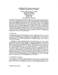
Fig. 1: Logarithmic Neuron In a single layer logarithmic network, the inputs are transformed to the natural logarithm (ln) of the input and the inverse natural logarithm (ln) is taken at the logarithmic neuron output. This method works well for the discussed cases but works poorly when additions and subtractions are involved. A two layer network whose first layer is composed of logarithmic neurons and whose output layer is a standard linear neuron remedies this problem. Figure 2 shows this two layer network. Logarithmic Neurons
x1
Linear Neuron
Σ x2 . xn
Σ
Σ w1
w2
f(x)
bias
Fig. 2: Two Layer Logarithmic Network The first layer of the logarithmic network transforms the inputs into functional terms. These terms are of the form:
term = x 1 w 1 ⋅x 2 w 2 L x n w n
(3)
The terms are then combined by the second layer of the network to form the function approximation.
2
f ( x ) = w 21 ⋅term1 + w 22 ⋅term2 + bias
(4)
Standard MLP networks could approximate this function, but it would require many nodes and it would only be valid over a range of inputs. This network architecture requires only one hidden logarithmic neuron for each term and is valid over all input values.
3. Network Training Training this network requires two choices: the correct objective function must be chosen, and a training algorithm must be chosen. This section explains the choice of objective function and derives the gradient descent based training algorithm. 3.1 Objective Function The standard MLP is trained to reduce the sum of the squared errors between the actual network output and the network target output for all of the training vectors. The SSE objective function is proper for classification problems but performs extremely poorly for function approximation problems that cover large ranges. A more correct objective function for function approximation is the sum of the percentage error squared (SPES). The SPES is the sum of the square of the percentage error between the target outputs and the actual outputs. It is defined in equation 5 with m equal to the number of training patterns.
1 SPES = 2
F F I (t − y ) I J G ∑ G H Ht KJ K 2
(5)
i =1,m
A difficulty with the SPES objective function is that the percentage error is undefined when the target vector is equal to zero. Therefore, training vectors must be chosen so that either the target vector is not equal to zero or a quick fix must be implemented. One such fix is to make those percentage error terms equal to the actual output. This will cause the SPES to increase when the actual output does not equal the target value of zero. 3.2 Training Algorithm The training algorithm attempts to minimize the objective function by changing the network weights. The standard backpropagation algorithm using gradient descent that became popular when published by Rumelhart and McClelland [7], can be easily manipulated to yield the correct weight update for the SPES objective function. The usual derivation uses the chain rule to find the updates with respect to the objective function. Using the chain rule and Haykin's [3] notation, the weight update for the output weights (wkj) is found to be
∆w kj = − ηo Where:
∂SPES ∂SPES ∂ek ∂yk ∂v k ek = − ηo = ηo yk = ηoδ k yk ∂w kj ∂ek ∂yk ∂v k ∂w kj t
wkj = ek = vk = yk = ηo = δ k =
(6)
weight from hidden neuron j to output neuron k. error signal at the output of output neuron k. internal activity level of output neuron k. function signal appearing at the output of output neuron k. the output layer learning rate. the local gradient.
To calculate the partial derivative of the objective function with respect to the hidden layer weights (wji), we again use the chain rule. Note the input layer is i, the hidden layer is j, and the output layer is k.
3
∂SPES ∂SPES ∂yj ∂v j = ∂w ji ∂yj ∂v j ∂w ji
(7)
This results in the local gradient term for the hidden neuron j:
δ j = exp( v j ) ′ δ ∑ kw kj = yj ∑ δkw kj k
(8)
k
and the hidden layer weight update is
∆w ji = ηhδ jy i = ηh yj ∑ δkw kj jyi ,
(9)
k
The change in the hidden layer weights is simply a backpropagation of the gradient terms back to the hidden layers through the output layer's weights taken into consideration the logarithmic transfer function. It is necessary to change the hidden layer errors using this procedure because there is no desired response from the hidden layer, but it is known that the hidden layer contributes to the error. The weight updates are completed in two stages. The first stage updates the output layer weights with its own variable learning rate (ηo) and the second stage updates the hidden layer weights with its variable learning rate (ηh). The learning rates increase when training successfully reduces the error and decrease when the error is not reduced by a weight update. Momentum is also included in the training algorithm through the standard formula.
4. Examples As an example, three hidden neurons were used to approximate the following function.
f ( x ) = 2. 3 ⋅x 12 − 1. 5 ⋅x 1 ⋅x 2 .5 + 4 ⋅x 2 2
(10)
The resulting weight matrices were w1 =
[0.9742 0.5292 2.0054 -0.0004 0.0025 1.9948]
w2 = [-1.5285
2.2420
4.1103].
This gives an approximate equation of
f ( x ) = 2. 24 ⋅x 12 − 1. 52 ⋅x 1.97 ⋅x 2 .52 + 4.11x 2 2 .
(11)
5. Comparison of Network Architecture Performances In this section the logarithmic-linear architecture described in this paper is compared with the standard MLP and the logarithmic transformation network. The logarithmic transformation network is a standard MLP network that uses the logarithmic transform of the input and target vectors for its input and target vectors. This allows it to operate in the logarithmic space. There are several limitations of this logarithmic transformation network. One is that neither the inputs nor the outputs can be negative. The network described in this paper, which we will now call the logarithmic-linear network, can have negative outputs. The second and most critical limitation is that the network has difficulties performing approximations for functions with more than one term as in example 1. Consider a function whose outputs are always positive.
4
f ( x ) = 2. 3 ⋅x 12 + 1.5 ⋅x1 ⋅x 2 .5 + 4 ⋅x 2 2
(12)
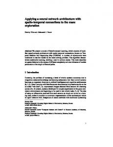
The test and training data: x1 and x2 ranged from .01 to 1000, resulting in outputs that ranges from 1x10⁻⁵ to 4x10⁶. The training set consists of 35 randomly chosen vectors that exercise most of the input space and the test set consists of 350 similarly chosen vectors. The standard MLP with a hyperbolic tangent hidden layer and a linear output layer was not able to reduce the mean percentage error below 100% with the number of hidden nodes ranging between 5 and 20. This inability to train shows that the MLP architecture is not suited to non-linear function approximation over large ranges. After training a logarithmic transformation network with 13 hidden nodes to an average error goal of 1%, the errors of the training set were plotted in Figure 3. A test set of random data from the same training interval was generated. This set is ten times larger than the training set and the errors are plotted in Figure 4. PERCENTAGE ERROR
PERCENTAGE ERROR
100
5
0
-100 0
-200
-300
-5 0
5
10
15
20
25
30
35
-400 0
40
Fig. 3: Logarithmic Transformation Network Training Set Errors
50
100
150
200
250
300
350
400
Fig. 4: Logarithmic Transformation Network Test Set Errors
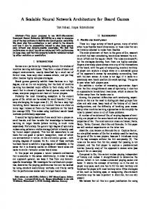
The same training set is used to train a logarithmic-linear network to a 1% error level resulting in the following weight matrices and the errors are plotted in Figure 5. Again, a ten times larger test set was generated on the same training intervals. The errors are plotted in Figure 6. w1 = [1.00623 0.4433 1.9946 0.0022 0.00177 1.9961]
w2 = [1.0819 2.3747 4.0854]
PERCENTAGE ERROR
PERCENTAGE ERROR
4
8
3
6
2
4
1
2
0
0
-1
-2
-2
-4
-3
-6
-4
-8
-5 0
5
10
15
20
25
30
35
-10 0
40
Fig. 5: Logarithmic-Linear Training Set Errors
50
100
150
200
250
300
350
Fig. 6: Logarithmic-Linear Test Set Errors
5
400
It is evident that both the logarithmic transformation network and the logarithmic-linear network can learn the training set to a high degree of accuracy. But the logarithmic-linear network generalizes much better. This is due to the network architecture being better suited to the structure of this type of non-linear function. It should also be noted that the logarithmic-linear network only used three hidden nodes while the purely logarithmic network required 13 hidden nodes to meet the 1% accuracy training requirement.
6. Summary This paper described a new neural network architecture that is better suited to non-linear function approximation than the both the standard MLP architecture and the logarithmically transformed MLP in some cases. The network makes use of a logarithmic hidden layer and a linear output layer. It can be trained to perform function approximations over a larger interval than both the standard MLP network and the logarithmic transformation network and can do it with significantly fewer neurons. This architecture can be thought of as an extension of the functional link network. It does not require the functions defined apriori, but learns them during training. This network architecture does have limitations. The current architecture does not support negative inputs. This may not be a limitation in real world problems where measured values are usually positive. And secondly, the number of terms must be known apriori or several networks with different numbers of hidden nodes must be constructed, trained, and their results compared. This limitation is common to most neural network architectures.
Acknowledgments The funding for this research provided by the Tennessee Valley Authority under contract number TV-93732V is acknowledged and was greatly appreciated.
References [1] Cybenko, G., 1989, Approximation by Superpositions of a Sigmoidal Function, Mathematics of Control, Signals, and Systems, 2, pp. 303-314. [2] Funahashi, K., 1989, On the Approximate Realization of Continuous Mappings by Neural Networks", Neural Networks, 2, pp. 183-192. [3] Haykin, S., 1994, Neural Networks, A Comprehensive Foundation, Macmillan, New York. [4] Hornick, K., Stinchcombe, M., and H. White, 1989, Multilayer Feedforward Networks are Universal Approximators, Neural Networks, 2, pp. 359-366. [5] Pao, You-Han, 1989, Adaptive Pattern Recognition and Neural Networks, Addison-Wesley, Reading, MA. [6] Pao, You-Han, Neural Networks and the Control of Dynamic Systems, IEEE Educational Video, ISBN: 07803-2258-4. [7] Rummelhart, D., E, eds., 1986, Parallel Distributed Processing: Explorations in the Microstructure of Cognition, Vol. 1, MIT Press, Cambridge, MA.
6