Sensor Errors Prediction Using Neural Networks A.Sachenko1, V.Kochan1, V.Turchenko1, V.Golovko2, J.Savitsky2, A.Dunets2, T. Laopoulos3 1
Research Laboratory of Automated Systems and Networks, Ternopil Academy of National Economy, 3 Peremoga Square, Ternopil, 46004, Ukraine, E-mail:
[email protected]
2
Laboratory of Artificial Neural Networks, Department of Electronics and Mechanics, Brest Polytechnic Institute, Moscowskaja 267, Brest, 224017, Belarus, E-mail:
[email protected]
3
Electronics Laboratory, Physics Department, Aristotle University of Thessaloniki, 54006, Thessaloniki, Greece, E-mail:
[email protected]
Abstract. The features of neural networks using for increasing of an accuracy of physical quantity measurement are considered by prediction of sensor drift. The technique of data volume increasing for predicting neural network training is offered at the expense of various data types replacement for neural network training and at the expense of the separate approximating neural network using. 1. Introduction In the majority of modern systems of sensor signals processing the measurement error of output sensor signal is normalized, instead of physical quantity. For example, at temperature measurement by sensor Honeywell Pt100 [1] and by unit Hydra 2625А Fluke [2] the errors ratio of the measuring channel elements is more than fifty. The majority of works on sensor signal processing [3, 4, 5] consider the questions which are not connected to increasing of sensor accuracy. The reliable increasing of the sensor accuracy is provides by it periodic testing with reference standard or calibration by using of the special calibrator on the exploitation place. But the operations realizing these methods are rather difficult [6]. The reduction of laboriousness is achieved by prediction of the sensor drift in intertesting interval [7]. In this case most effective is using of an artificial intelligence methods, in particularly, neural networks [8, 9, 10]. It is known [11] that the quality of neural networks training depends on volume of data used for training in strong degree. It causes a main contradiction of neural networks using for sensors drift correction. The high-quality neural network training allows sharp reducing the prediction error. It allows increasing of an intertesting interval that obtained by testing or calibration volume of data will appear insufficient for highquality neural networks training. For solution of this contradiction, that is for artificial increasing of the training points number for predicting neural network it is offered to use historical data (data of drift of the same type sensors in the similar exploitation conditions) [10] and additional approximating neural network [12]. It is most expedient to share usage of these methods. Obviously, that the best prediction quality is provided by training of the predicting neural network on real data about sensor drift (obtained by testing or calibration). Therefore, the real data should replace the historical data in accordance with accumulation of real data during sensor exploitation. Features of artificial increasing of training points number for predicting neural network by offered methods are considered below. 2. Method of Replacement of Historical Data by Real Data Let us consider the historical data of sensors drift as curves d 1 ...d n (see Fig. 1), which in moments of calibrations a , b, c are equal to d i a , d i b , d i c , i = 1, n . The first calibration of the new sensor in moment a allows receiving the first real value d k a . The purpose of the historical data using is the prediction of number of points d k b , d k c on the basis of d k a and etc. that allow to predict drift of the sensors in the moments of future calibrations. For this purpose it is expedient to use the separate neural network, which should predict point d k b on the basis of d k a and d i a , i = 1, n , the next point d k c on the basis of d k b and d i b , i = 1, n and etc. The number of available historical curves of sensor drift determines a structure of input layer of neural network. For prediction it is expedient to apply the model of single-layer perceptron with linear activation function of neuron. The output value of perceptron 441 0-7695-0619-4/00/$10.00 © 2000 IEEE
y=
n
∑ wi1 xi − T
,
(1)
i =1
where wi1 are the weight factors of inputs of linear neuron, xi is the input data, T is the neuron’s threshold.
Fig. 1. Historical Data about drift of same type sensors
For perceptron training was used Widrow-Hoff rule [13]. The total sum-squared error of training is E=
L
L
1
∑ E (k ) = 2 ∑ ( y k − d k ) 2 , k =1
(2)
k =1
where L is set of training vectors, E (k ) is the sum-squared error for k input vector, y k , d k are the output and desirable values for k input vector accordingly [14]. The final expressions for weight factors and thresholds modification is wi1 (t + 1) = wi1 (t ) − α (t )( y k − d k ) xi k , T (t + 1) = T (t ) + α (t )( y k − d k ) ,
(3)
where i = 1, n , xi k – i is the component of k vector, α (t ) = 1 +
xi (t ) i =1 n
∑
2
−1
(4)
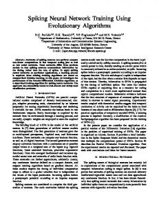
is an adaptive learning rate. The following algorithm is used for training [14]: 1. Set the adaptive learning rate α (0 < α < 1) and minimal sum-squared error Emin , which it is necessary to achieve at training; 2. Initialize the weight factors and threshold of neural network by a casual law; 3. Give an input data on the neural network input, to calculate the outputs according to expression (1); 4. Update the values of weight factors and threshold of neural network according with expressions (3), (4); 5. Execute steps 3-4 so long as total sum-squared error (2) will not become less minimal E ≤ E min . The prediction of sensor drifts after calibrations b, c etc. is carried out by shift to right on one calibration (see Fig. 1) of all necessary data for forming of training vectors set. 3. Models of an Approximating and Predicting Neural Networks As approximating neural network is used three-layer perceptron consist of one input neuron, hidden layer of neurons and one output linear neuron (Fig. 2а). The output value of three-layer perceptron is
442
Nh
YO = ∑ wi 0 hi − s0 ,
(5)
i =1
where N h is the number of neurons of hidden layer, wi 0 is the weight from i - neuron to output neuron, hi is the output of i - neuron, s 0 is the threshold of i - neuron.
Y
h Nr −h1
h1
h1r −1
YO
h2
xI
r −1
Z-1 Z-1
Z-1
h1r x1p
hN
Y p (t )
h
x Nr I
h Nr h
a)
b)
Fig. 2. Structures of approximating (a) and predicting (b) neural networks
The output value of the neurons of hidden layer is h j = g (wIj xI + s j ) ,
(6)
where wIj is the weight from input neuron to j - neuron of hidden layer, xI is the neuron’s value of input layer, s j are thresholds of hidden layer neurons. For neurons of hidden layer the logistic activation function is used
(
)
−1
g ( x ) = (1 + e − x . (7) For training of an approximating neural network is used the algorithm of back propagation error [15]. It is based on the gradient descent method and consists of fulfillment of an iterative procedure of updating weights and thresholds for each training vector p from training set ∆wij (t ) = −α
where α is the learning rate,
∂E p (t ) , ∂wij (t )
∆s j (t ) = −α
∂E p ( t ) , ∂s j ( t )
(8)
∂E p ( t ) ∂E p ( t ) , are gradients of the error function on training iteration t for training ∂wij (t ) ∂s j (t )
vector p , p ∈ {1, P} , P - size of training set.
(
)
2 1 p YO (t ) − DOp , 2 p where YO (t ) is the output value of the neural network on iteration t for training vector p , DOp - desirable value of network output for training vector p . During training the total error is reduced
E p (t ) =
P
E (t ) =
∑E p =1
443
p
(t ) .
(9)
With the purpose of improving of neural network training parameters and removing of classical back propagation algorithm’s defects connected with empirical choice of learning rate we use the steepest descent method for calculation of learning rate [12]. Thus, the adaptive learning rate for logistic activation function is Nh
αˆ p (t ) =
(
1
)
×
∑ (γ jp (t ))2 h jp (t )(1 − h jp (t )) j =1
Nh p 2 p 2 ∑ (γ j (t )) (h j (t )) (1 − h jp (t ))2 j =1 p where γ j (t ) is an error of j - neuron for logistic function for training vector p , 1 + ( xIp ) 2
,
(10)
and for linear activation function
α p (t ) =
1 Nh
∑
,
(11)
( hip (t )) 2 + 1
i =1
where
hip (t )
are an input signals of linear neuron on training iteration t for training vector p . Nh
γ ip (t ) = ∑ γ 0p (t ) wi 0 (t )h jp (t )(1 − h jp (t )) ,
(12)
j =1
where wi 0 (t ) are weight factors from neurons of the hidden layer to output neuron adapted on training iteration t , (13) γ 0p (t ) = Y0p (t ) − Dop . At neural network training the problem of weight factors initialization is rather actual. The speed, accuracy and stability of training depend on it largely. Usually initialization is setting to neuron weights and thresholds the casual uniformly distributed values from range: wij = R( c, d ), s j = R (c, d ) . The upper and lower boundaries of this range are defined empirically. We offer to use the mathematical approach for calculation of the boundaries of weight initialization that allows essentially reducing training time [12]. For stabilization of training process the algorithm of level-by-level training has been used: 1. Calculate the upper and lower boundaries of weight range for neurons of hidden layer and for output neuron and initialize weights and thresholds of neurons; 2. For training vector p calculate the output value of network YO p (t ) using expressions (5, 6); 3. Calculate an error of output neuron (13); 4. Update weights and thresholds of output neuron (8) using an adaptive learning rate (11); 5. Calculate an error γ jp (t ) of neurons of hidden layer for network with updating weights of output layer (12) for logistic activation function (7); Update weights and thresholds of neurons of the hidden layer (8) using an adaptive learning rate (10) for logistic activation function; 7. Execute steps 2-6 so long as the total training error of the network (9) will not become less required. The application of the given algorithm allows stabilizing perceptron training process with various neurons’ activation functions and considerably reducing training time. As predicting there is used three-layer recurrent neural network containing one hidden layer of nonlinear neurons and one linear output neuron (Fig. 2b). The output value of neural network is 6.
Nh
Y r = ∑ wi 0 hir − s0 ,
(14)
i =1
where N h is the number of neurons of hidden layer, hir are the output values of neurons of hidden layer in moment r , s 0 is the threshold of output neuron, wi 0 are weights from i - neurons to output neuron. The output value of neurons of hidden layer in moment r for training vector p NI
Nh
∑w x + ∑ w h
h rj = g (
r ij i
i=1
k =1
444
r −1 kj k
+w0 j Y r −1 + s j ) ,
(15)
where N I is the size of input vector, wij are weights from i input neurons to j neurons of hidden layer, xir is the i - element of input vector x r , wkj are weights from k - neurons to j -neurons of hidden layer, hkr −1 (t ) is the
output of the k -neuron in previous moment of time r − 1 , w0 j are weights to neurons of hidden layer from output neuron, Y r−1 (t ) is the output network value in the previous moment of time r − 1 , s j are thresholds of neurons of hidden layer. The logistic activation function (7) and logarithmic activation function (16) g ( x ) = ln ( x + x 2 + a ) a , (a > 0) are used as activation function of neurons of hidden layer in predicting neural network. The function (15) is unlimited on all area of definition. It allows better simulating and predicting complicated non-stationary processes. The parameter a determines declination of activation function. For logistic function (7) an adaptive learning rate is Nh
αˆ p (t ) =
1
×
∑ (γ jp (t ))2 h jp (t )(1 − h jp (t )) j =1
1 + ∑ ( xip ) 2 + ∑ (hkp−1 (t ))2 + (Y p−1 (t )) 2 ∑ (γ jp (t ))2 (h jp (t )) 2 (1 − h jp (t ))2 k =1 i=1 j =1 where γ jp (t ) is the error of j -neurons with logistic activation function for training vector p NI
Nh
Nh
Nh
γ ip (t ) = ∑ γ 0p (t ) wi 0 (t )h jp (t )(1 − h jp (t )) .
,
(17)
(18)
j =1
For logarithmic function (15) an adaptive learning rate is Nh
αˆ p (t ) =
1 1 + ∑ ( xip ) 2 + ∑ ( hkp −1 (t )) 2 + (Y p −1 (t )) 2 k =1 i =1 NI
NI
Nh
i =1
k =1
Nh
×
a ∑ (γ jp (t )) 2 ( B jp (t )) 2 + a j =1
(
Nh p ∑ (γ j (t )) 2 ( B jp (t )) 2 + a j =1
)
−1
−1
,
(19)
where B jp (t ) = ∑ wij (t ) xip + ∑ wkj (t )hkp−1 (t ) +w0 j (t )Y p−1 (t ) + s j is the weighted sum of j - neurons’ inputs of hidden layer, γ jp (t ) is the j - neuron error for training vector p calculated on each training iteration t : Nh
1
j =1
1 + ( B jp (t )) 2
γ ip (t ) = ∑ γ 0p (t ) wi 0 (t )
.
(20)
An adaptive initialization of weights and thresholds [12] and defined above algorithm of level-by-level training with expressions (14-20) are used in predicting neural network also. 4. Experimental Researches The training vectors for data replacement are obtained from 10 curves of historical drifts of sensors. At training of 10-inputs single-layer perceptron the sum-squared error 10Е-7 is reached. All diagrams of percentage errors of historical data replacement after 5 calibrations are presented in Fig. 3a. The percentage error of data replacement exceeds 10% only in one case. For estimation of approximating neural networks the 5 points of historical data calibrations are used. At training of the model with 5 hidden neurons and activation function (7) the sum-squared error 2.4Е-7 is reached. In Fig. 3b the maximum and average percentage errors of approximations in 5 points of calibrations are presented. The maximum percentage error does not exceed 2%. The result of approximation contains 25 points on each curve of historical data after which predicting neural network (model with 10 input neurons, 10 hidden neurons with activation function (7), and one output linear neuron) was trained. The results of prediction (maximum and average percentage errors) for sum-squared error of training 7.8Е-8 are presented in Fig. 3b. As it is seen from figure the offered methods allow increasing an intertesting interval in 10 times at allowable prediction error 11%.
445
Conclusion The exploitation features make difficult direct use of artificial intelligence methods, in particularly, neural networks for accuracy increasing of the sensor signal processing systems. The offered methods will allow providing sharper reduction of error of physical quantity measurement at the expense of high adaptability of intelligent systems. These methods are best for using in distributed hierarchical systems [16, 17] where the neural network training is performed on a higher system’s level and prediction is performed on lower levels. Acknowledgement Authors would like to thank INTAS, grant reference number INTAS-OPEN-97-0606.
a)
b)
Fig. 3. Percentage errors of replacement (a) and approximation and prediction (b)
References [1] [2] [3] [4] [5] [6] [7] [8] [9] [10] [11] [12] [13] [14] [15] [16] [17]
http://www.honeywell.com/sensing/prodinfo/temperature/catalog/c15_93.pdf www.fluke.com/products/data_acquisition/hydra/home.asp?SID=7&AGID=0&PID=5308 Iyengar S.S., “Distributed Sensor Network - Introduction to the Special Section”, Transaction on Systems, Man and Cybernetics, vol. 21, No. 5, 1991, pp 1027-1035 Finkelstein L., “Measurement and instrumentation centre”, Measurement, vol. 14, No 1, 1994, pp.23-29. Sydenham P.H., “Sensing Science and Engineering Group”, Measurement, vol 14, No 1, 1994, pp.81-87 Brignell J., “Digital compensation of sensors”, Scientific Instruments, vol. 20, No 9, 1987, pp.1097-1102 Sachenko A., “Development of accuracy increasing methods and creation of precision systems of temperature measurement in industrial technologies”, Dr. Techn. Sci. Thesis, Leningrad, 1988, 32p. C.Alippi, A.Ferrero, V.Piuri, “Artific. Intelligence for Instruments & Applications”, IEEE I&M Magazine, Jun’98, pp.9-17. P. Daponte, D. Grimaldi, “Artificial Neural Networks in Measurements”, Measurement, vol. 23, 1998, pp.93-115. Golovko V., Grandinetti L., Kochan V., Laopoulos T., Sachenko A., Turchenko V., “Sensor Signal Processing Using Neural Networks”, IEEE Region 8 Intern. Conf. Africon’99, Cape Town (South Africa), 1999, pp.345-350. Kroese B., “An Introduction to Neural Networks”, Amsterdam, University of Amsterdam, 1996, 120p. V.Golovko, J.Savitsky, A.Sachenko, V.Kochan, V.Turchenko, T.Laopoulos, L.Grandinetti, “Intelligent System for Prediction of Sensor Drift”, Proc. Intern. Conf. Neural Networks and AI ICNNAI’99, Brest (Belarus), 1999, pp.126-135. Widrow B., Hoff M., “Adaptive Switching Circuits”, In 1960 IRE WESCON Conv. Record, DUNNO, 1960, pp.96-104. A.Sachenko, V.Kochan, V.Turchenko, V.Tymchyshyn, N.Vasylkiv, “Intelligent Nodes for Distributed Sensor Network”, Proceedings of 16th IEEE Instrumentation and Measurement Tech. Conf. IMTC/99, Venice (Italy), 1999, pp.1479-1484. Rumelhart D., Hinton G., Williams R, “Learning Represent. by Backpropag. Errors”, Nature, 1986, No 323, pp.533-536. A.Sachenko, V.Kochan, V.Turchenko, “Intelligent Distributed Sensor Network”, Proceedings of 15th IEEE Instrumentation and Measurement Tech. Conf. IMTC/98, St. Paul (USA), vol.1., 1998, pp.60-66. V.Golovko, L.Grandinetti, V.Kochan, T.Laopoulos, A.Sachenko, V.Turchenko, V.Tymchyshyn, “Approach of an Intelligent Sensing Instrumentation Structure Development”, Proc. of IEEE International Workshop on Intelligent Signal Processing WISP’99, Budapest (Hungary), 1999, pp.336-341.
446