Chapter 32
A Logistic Based Cellular Automata Model for Continuous Urban Growth Simulation: A Case Study of the Gold Coast City, Australia Yan Liu and Yongjiu Feng
Abstract This chapter presents a logistic based cellular automata model to simulate the continuous process of urban growth in space and over time. The model is constructed based on an understanding from empirical studies that urban growth is a continuous spatial diffusion process which can be described through the logistic function. It extends from previous research on cellular automata and logistic regression modelling by introducing continuous data to represent the progressive transition of land from rural to urban use. Specifically, the model contributes to urban cellular automata modelling by (1) applying continuous data ranging from 0 to 1 inclusive to represent the none-discrete state of cells from non-urban to urban, with 0 and 1 representing non-urban and urban state respectively, and all other values between 0 and 1 (exclusive) representing a stage where the land use is transiting from non-urban to urban state; (2) extending the typical categorical data based logistic regression model to using continuous data to generate a probability surface which is used in a logistic growth function to simulate the continuous process of urban growth. The proposed model was applied to a fast growing region in Queensland’s Gold Coast City, Australia.
32.1
Introduction
This chapter presents a logistic based cellular automata model to simulate the continuous process of urban growth in space and over time. The model is constructed based on an understanding from empirical studies that urban growth is a continuous spatial
Y. Liu (*) Centre for Spatial Environmental Research and School of Geography, Planning and Environmental Management, The University of Queensland, Queensland, Australia e-mail:
[email protected] Y. Feng College of Marine Sciences, Shanghai Ocean University, Shanghai, P. R. China
A.J. Heppenstall et al. (eds.), Agent-Based Models of Geographical Systems, DOI 10.1007/978-90-481-8927-4_32, © Springer Science+Business Media B.V. 2012
643
644
Y. Liu and Y. Feng
diffusion process over time which can be described through the logistic function (Herbert and Thomas 1997; John et al. 1985; Jakobson and Prakash 1971). It extends from previous research on cellular automata and logistic regression modelling by introducing continuous data to represent the progressive transition of land from rural to urban use. Specifically, the model contributes to urban cellular automata modelling by (1) applying continuous data ranging from 0 to 1 inclusive to represent the nonediscrete state of cells from non-urban to urban, with 0 and 1 representing non-urban and urban state respectively, and all other values between 0 and 1 (exclusive) representing a stage where the land use is transiting from non-urban to urban state; (2) extending the typical categorical data based logistic regression model to using continuous data to generate a probability surface which is used in a logistic growth function to simulate the continuous process of urban growth. The proposed model was applied to a fast growing region in Queensland’s Gold Coast City, Australia. Many CA based urban models have been developed over the last two decades (see Iltanen 2012); these models vary considerably based on the configurations of the five basic elements that make up the CA model – the type and size of the cells, the definition of cell states, the type and size of the neighbourhood, the configuration of transition rules, and the way time is modelled. While the sizes of cells and their neighbourhood are fundamentally a scale issue which is common to all geographical problems (Openshaw 1984), it is more challenging for modellers to configure the state of the cells and identify rules that drive the transition of cells from one state to another over time in order to capture the various features and mechanisms of urban growth dynamics. A common practice in defining cell state is using discrete data to represent a binary state of either non-urban or urban, or using specific land use types (Ward et al. 2003; Li and Yeh 2000; Clarke and Gaydos 1998; Wu 1998a, b, c, 1996; Clarke et al. 1997). Many of these models have made significant contributions to our understanding on urban growth and land use change dynamics both theoretically and empirically, however, a limitation of this modelling practice is in capturing the progressive or continuous change of state geographically and temporally. To overcome this limitation, Liu (2008) and Liu and Phinn (2003) developed models using a fuzzy membership function to represent the fuzzy boundary between the urban core and suburb areas towards the rural land. Other models developed by Mandelas et al. (2007), Dragićević (2004) and Wu (1998b) also introduced the fuzzy set and fuzzy logic concepts in their models following the pioneering attempt by Wu (1996). However, as the membership function and the fuzzy linguistic modifiers are defined in a subjective way, the interpretation of the model’s results is largely restricted (Wu 1996). In terms of identifying and configuring the transition rules, both statistical and non-statistical methods have been developed; the former include the Monte Carlo method (Clarke et al. 1997), the analytical hierarchy process (AHP) (Wu 1998c), multi-criteria evaluation (MCE) (Wu and Webster 1998), principal components analysis (PCA) (Li and Yeh 2002a), multiple regression analysis (Sui and Zeng 2001), and logistic regression (Wu 2002); and the latter include the artificial neural network (Almeida et al. 2008; Li and Yeh 2002b), and the spatial optimization methods such as particle swam optimization (Feng et al. 2011), support vector
32
A Logistic Based CA Model for Continuous Urban Growth Simulation
645
machines (Yang et al. 2008), kernel method (Liu et al. 2008a), and ant intelligence (Liu et al. 2008b). Amongst these approaches, the logistic regression method has been favoured in a number of studies primarily due to its strong statistical foundation in exploring the association of a dependent variable, measured as presence or absence of a phenomenon (e.g., yes/no, or urban/non-urban), and multiple independent (predictor) variables such as the various environmental, social and institutional factors on urban growth. For instance, Wu and Yeh (1997) applied logistic regression method for modelling land development patterns based on parcel data extracted from aerial photographs; Gobim et al. (2002) adopted logistic modelling technique to predict the probabilities of local agricultural land use systems in Nigeria; Wu (2002) used logistic regression to compute the probability of a cell experiencing land change and developed a stochastic CA model; Verburg et al. (2002) developed a spatially-explicit land-use change model (i.e. CLUE-S) based on logistic regression to simulate land-use change in relation to socio-economic and biophysical driving factors, which has also been widely applied in other areas (e.g., Zhu et al. 2009); Fang et al. (2005) used logistic regression to analytically weigh the scores of the driving factors of an urban sprawl model for predicting probability maps of land use change. Indeed, the logistic regression method is effective and efficient in modelling urban growth with cellular automata. However, the use of categorical data representing a binary state of non-urban or urban is limited in modelling areas that are partly developed but are yet to be fully urbanised. Given that the logistic regression model is not restricted to only using categorical data to represent the dependent variable, this method can also be applied to model continuous dependent variable data, so long as the data is within a range from 0 to 1 representing probability values or proportions (Sherrod 2010). The following section describes the study area where the proposed logistic CA model using continuous data will be tested and calibrated, followed by a section on model description, including the model design concepts and principles, input data and the model configuration details. The results generated from the application of the model in simulating the processes of urban growth in the Gold Coast City from 1996 to 2006 are presented and discussed in the Results section, together with assessments of the model’s simulation accuracies using a set of landscape matrix measures. The last section of the chapter summarises findings from the current research and identifies future research directions.
32.2
Study Area
Gold Coast City, the second largest city in Queensland, Australia was selected to apply the logistic regression based CA model to simulate the continuous urban growth from 1996 to 2006. Geographically, the city is situated in the southeast corner of Queensland between the state’s capital city of Brisbane at its north and the State of New South Wales at its south. To the west of the Gold Coast are
646
Y. Liu and Y. Feng
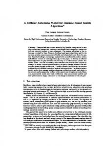
Fig. 32.1 The study area
the Lamington National Park and the foothills of the Great Dividing Range. Spanning across an area of 1,400 km2 and with 57 km of coastline, this city has some of the most popular surf breaks and beaches in Australia and the world; its west and southwest hinterland also offers the most spectacular scenery in Australia and extremely rich biodiversity which supports rural production, water quality, scenic amenity and outdoor recreation (Department of Infrastructure and Planning 2009). This city consists of 106 state suburbs prior to the year 2008, with a number of localities, towns and rural districts within the suburbs. Since March 2008, Beenleigh-Eagleby region on Gold Coast’s northwest border has been transferred to Logan City. Given that the time frame in this study is from 1996 to 2006, the study area still includes those suburbs that are currently part of Logon City (Fig. 32.1). The total resident population of the city in 2006 was 472,000 (Australia Bureau of Statistics 2006), and the estimated resident population in 2010 was 528,000 (Australian Bureau of Statistics 2011). Over the past 15 years, the urban
32
A Logistic Based CA Model for Continuous Urban Growth Simulation
647
footprint has been growing rapidly with most of development been concentrated between Yatala at the north and Coolangatta at the south, and continues south beyond the Queensland border into the Tweed Shire in New South Wales (Department of Infrastructure and Planning 2009; Ward et al. 2000).
32.3
Model Description
The model description follows the ODD (Overview, Design concepts, and Details) protocol for describing individual- and agent-based models (Grimm et al. 2006, 2010; Grimm and Railsback 2005, 2012) and consists of seven elements. The first three elements provide an overview of the model; the fourth element explains general concepts underlying the model’s design; and the remaining three elements provide details.
32.3.1
Purpose
The purpose of the model is to simulate urban growth as continuous processes in space and over time. It hypothesises that the transition of land from rural to urban use is a continuous process which can be modelled using continuous data and logistic functions in a cellular environment. The proposed cellular model was applied to the rapidly growing Gold Coast City in Southeast Queensland, Australia to test the conceptual framework and effectiveness of the model in simulating the continuous processes of urban growth.
32.3.2
Entities, State Variables and Scales
In cellular automata based urban modelling, the space or area under study is typically tessellated into regular grid cells, each cell representing a piece of land on the ground at a certain scale. For the study area in the Gold Coast City, the spatial scale of cells is at 30 m, with a total of 1,559,283 cells covering the entire study area. Each spatial entity or cell is represented by a state variable representing the state of a cell undertaking the urban development process. Instead of defining the state variable with a binary value of urban or non-urban, as most other CA based urban models typically do, this model defines the state of cells as continuous values ranging from 0 to 1 (inclusive). For instance, a non-urban cell which has not started its development will have a state value of 0, while a fully developed urban cell will have a state value of 1. Cells that have started their process of urban development but are yet to be fully developed will have a state value between 0 and 1 (exclusive). Another state variable used in the CA model is the neighbourhood size. In this study, a rectangular 5 × 5 cells neighbourhood was selected. According to CA
648
Y. Liu and Y. Feng
Fig. 32.2 The logistic urban growth process under various growth control speeds
principles, the state of a cell at a certain time is not only dependent on the state of the cell itself in a previous time step, but also the collective effect of all cells within its neighbourhood. This collective neighbourhood effect is modelled in the land use conversion probability sub-model.
32.3.3
Process Overview and Scheduling
Three processes of urban growth have been modelled; these include a continuous urban growth process, a new urban growth process, and a no-growth process. All processes are under the assumption that urban growth progress from a lower state (with a state value close to 0) to a higher state (with a state value close to 1), with the value 1 being the highest state in the urban growth process. Once a cell reaches a state value of 1, it is considered being fully developed and its state will remain as 1 until the simulation is terminated. This excludes both urban re-development and anti-urbanisation processes. Continuous urban growth The continuous process of urban growth can be represented by a logistic function (Liu 2008; Herbert and Thomas 1997; John et al. 1985; Jakobson and Prakash 1971). Sit =
1 1 + (1 / S0 - 1) ´ exp ( -g ´ t )
(32.1)
where Sit is the state of cell i at time t; S0 is the initial state of the cell to start its urban growth process. This initial state value can be small but larger than 0 for the cell to start its urban growth process (e.g., S0 = 0.01 ). g is a parameter ranging from 0 to 1 which controls the speed of the urban growth process (Fig. 32.2).
32
A Logistic Based CA Model for Continuous Urban Growth Simulation
649
This growth control parameter is modelled through a land use conversion probability sub-model, which will be discussed further in the Design Concept and Sub-model sections. New growth A new growth process can occur to a non-urban cell if there is a high probability for such growth to occur. For instance, if a non-urban cell is surrounded by cells which are all fully urbanized, this non-urban cell may have the tendency or be influenced by its neighbouring cells to develop towards an urban state. In this case, an initial very low value is assigned as the state of the cell so it can start its urban growth process. Once a non-urban cell is triggered to start its urban growth process, it will then follow the continuous urban growth process; the growth speed is also controlled by the land use conversion probability at the time of development. No growth Apart from the above two growth processes, other non-urban cells will remain as nonurban until such conditions where new development can be triggered to proceed. Model scheduling The model starts from a historical time where input data is available to represent the initial state of entities in the model. For the City of Gold Coast, this starting date was set to 1996. Another set of data was collected in 2006 which was used to calibrate the model over time. The temporal iteration of the simulation process was determined by comparing the overall urban area generated by the model with the actual urban area size in 2006; if the generated urban area size is within less than 1% difference from the actual urban area size in 2006, then the model is terminated for a simulation accuracy assessment in 2006. This calibration process continues until satisfactory results were achieved which match with the actual urban growth patterns.
32.3.4
Design Concepts
Basic principles: The basic principle imbedded in this urban cellular model is that urban growth is a continuous spatial diffusion process overtime. Spatially, an urban area is featured with high population density and the dominance of nonagricultural land. However, as cities are surrounded by rural or natural land, there is no clear boundary between an urban built-up area and its non-urban hinterland. Between the well-recognized urban land use and the area devoted to agriculture, there exists ‘a zone of transition in land use, social and demographic characteristics, lying between (a) the continuously built-up area and suburban areas of the central city, and (b) the rural hinterland, characterized by the almost complete absence of non-farm dwellings, occupations and land use’ (Pryor 1968:206). This ‘zone of transition’ is a place where both urban and non-urban features occur, which has been broadly termed as ‘fringe’ or ‘rural-urban fringe’ (Bryant et al. 1982; Pryor 1968). The urban fringe area has become the most vigorous part of
650
Y. Liu and Y. Feng
development in the rural-urban continuum and has attracted much attention in research. Temporally, the transition of land from rural to urban use is a continuous process which occurs over a period of time. This transition process can be illustrated through a logistic function with five distinctive growth stages which can be illustrated by Rostow’s five-stage model of development, Which can be illustrated by Rostow’s five-stage model of development, that is, it transits from a traditional rural society to pre-conditional stage for growth. Which can be illustrated by Rostow’s five-stage model of development, to a take-off stage for rapid growth, and then to a drive to maturity stage and a final stage of urban society (Potter et al. 2003). Such spatial and temporal processes of continuous growth cannot be captured through a conventional CA model with binary states of non-urban and urban configurations. While the general process of urban growth can be described through a logistic growth function, the speed of such growth or any possibility of new growth are affected by a number of other factors, namely, the neighbourhood effect, accessibility to infrastructures and services, physical or institutional constraints on the use of land, and other stochastic factors that are uncertain at time of modelling. Such impact factors can be built into the logistic function through a probability index at individual cell scale. This probability index is computed in a sub-model which is elaborated further in the Sub-model section. Emergence: Urban growth patterns emerge from the transition of states of individual cells, but the transition of individual cells from one state to another is dependent on the state of the cell itself and the states of neighbouring cells at a previous time step according to certain transition rules. Adaptation: The transition of land use from non-urban to urban is an adaptive process over time; each cell will adapt to change of the land use conversion probability according to its environmental conditions. For instance, a cell with a high probability for growth will develop faster than those with lower probability for growth. A high land use conversion probability is related to advantageous driving factors such as close proximity to transportation network, facilities and services or strong neighbourhood support. On the other hand, a low land use conversion probability is more likely associated with lack of support for growth or other land use constraint, such as steep slope or other planning constraints. Objectives: The objective of the model is for the simulated patterns of urban growth to match the actual pattern of urban growth at certain point in time. For instance, if the model is initialised with the actual urban growth data in 1996 to generate the urban growth scenario in 2006, the objective of the model is for the simulated urban growth scenario in 2006 to match with the actual urban growth patterns at that point in time. Learning: Individual cells may change their transition speed over time as a consequence of their experience in matching the expected state of the cell during the model calibration process.
32
A Logistic Based CA Model for Continuous Urban Growth Simulation
651
Prediction : Under the basic principle that urban growth will progress continuously from a lower to a higher state over time, it is assumed that individual cells are able to predict their cell state in this growth process according to the logistic function. However, this predictability is inherently associated with their adaptability to change of the land use conversion probabilities in space and over time. Sensing: Individual cells are assumed to know their own state and the state of their neighbouring cells. They can also sense the environmental conditions such as land slope, spatial proximity to urban centres, and other data regarding the socioeconomic and environmental conditions. Interaction: Interaction amongst cells is modelled through the neighbourhood effect. In essence, the collective state of all cells within the neighbourhood of a processing cell contributes significantly to the land use conversion probability index, which in turn impact on the transition speed of the cell in its urban growth process. Stochasticity: The land use conversion probability sub-model includes a stochastic disturbance factor on urban development. This stochastic factor is used to represent any unknown or unexpected factors that may impact on land use conversion probability, hence reproduce variability in the simulation processes. Collectives: The impact of neighbourhood effect on urban growth is modelled collectively. The mean state value of all cells within the neighbourhood of the processing cell will impact on the land use conversion probability which is modelled through the land use conversion probability sub-model. Observation: Observations of the model’s results include graphical display of urban patterns in space and over time. For model calibration, results generated by the model were compared with the actual urban growth patterns through a set of landscape metrics and a spatial confusion matrix analysis.
32.3.5
Initialization
Each cell in the cellular space was initially assigned a state value ranging from 0 to 1 inclusive representing its state in the urban growth process. This initial state value was assigned based on the modified population density map computed from the 1996 Census of Population and Housing data at the Census Collection District (CCD) level; the modification was carried out using the 2006 Census data at the mesh block level (Australian Bureau of Statistics 2005, 2006). As the mesh block data contains higher spatial resolution than the 1996 data at the CCD level, areas identified as non-urban in the 2006 mesh block data were projected back to the 1996 census data to define the area as non-urban in 1996, if the area was not identified as non-urban with the 1996 census data. This modification increases the spatial accuracy of the initial input data for the model to commence.
652
32.3.6
Y. Liu and Y. Feng
Input Data
The input data used in the model include two sets of census data in 1996 and 2006. The 1996 census data were processed at CCD level and used (with modification as elaborated above) to define the initial state of the cells in the cellular space. The 2006 census data were collected at the mesh block level to modify the 1996 census data in order to increase the spatial accuracy of the population density map; this dataset was also used to define the state of cells in 2006 which were used subsequently to calibration the simulation accuracy of the model. In addition, a set of spatial proximity or distance variables were also generated to feed the logistic regression model which was used to generate the land use conversion probability due to spatial proximity to facilities and services. Data defining the continuous state of cells Two threshold values were used to define the lower and upper limits of population density respectively in delimiting the cell state in the urban growth process. These threshold values were set to 200 and 1,500 persons per square kilometres respectively; this reflects the relatively low population density measure used in Australia to delimit the extent of urban areas (Liu 2008; Linge 1965). A cell with a population density of less than 200 persons per square kilometre is defined as non-urban; its cell state is assigned a value of 0. Similarly, a cell with a population density of 1,500 persons per square kilometre or over is defined as urban; its cells state is assigned a value of 1. All other areas with a population density value of between 200 and 1,500 persons per square kilometre is assigned a state value between 0 and 1, which are linearly interpolated based on the density value of the cell at the specified point in time. Other input data The constraint data to urban growth used in the model includes transportation network such as highways, primary and secondary roads, data identifying the major urban and town centres, land use planning schemes, and data illustrating areas where urban development cannot occur, such as large water bodies, forest reserves, nature conservation reserves, large recreational areas, prohibited areas for defence purpose, mine sites, golf courses and major aquaculture areas. These data were collected from various government agencies and processed as raster data in GIS at 30 m spatial scale. While many spatial factors may impact on urban land use change, in practice, not all factors can be quantified into a simulation model, especially when data reflecting such factors are neither available nor accessible. Historically, Gold Coast’s urban growth has been largely driven by existing urban and town centres and the spatial accessibility to transportation and other infrastructure and services; it is also constrained by natural conservation and primary agricultural land. Therefore, eight spatial factors reflecting the spatial proximity of each cell to urban and town centres, to main roads, to residential, industrial, commercial and educational areas, and to natural conservation and primary agricultural land,
32
A Logistic Based CA Model for Continuous Urban Growth Simulation
Table 32.1 Variable dct drd drs din dco ded dpk dag PN C
R
653
Variables used to compute land conversion probability Meaning Data extraction Distance to urban and town centres Distance variables were extracted from various GIS data layers including Distance to main roads urban centres, transportation Distance to residential areas network, coastal lines and land use Distance to industrial areas data layers Distance to commercial areas Distance to educational areas Distance to parkland Distance to agricultural land Probability of a cell changing from non-urban to urban within a rectangular 5 × 5 cells neighbourhood Land use constraints including large water bodies, forest reserves, nature conservation reserves, large recreational areas, prohibited areas for defence purpose, mine sites, golf courses and major aquaculture areas as well as land use restrictions through planning regulation A stochastic disturbance factor representing any unknown errors
Calculated using GIS’s focal function
Extracted from urban land use and planning data
Randomly generated in GIS
together with the neighbourhood effect, physical and land use zoning constraints, and a stochastic disturbance factor representing any unexpected errors on urban growth to simulate the continuous processes of its urban development (Table 32.1).
32.3.7
Sub-model
32.3.7.1
Land Use Conversion Probability Sub-model
While urban development follows the logistic function in general, the speed of development varies from one location to another within the urban cellular space over time. This factor is reflected in Eq. 32.1 through the parameter of γ . This parameter can be represented by a land use conversion probability which is determined by the collective effect of its spatial proximity to other facilities and services, the neighbourhood effect, land use suitability constraints as well as a stochastic disturbance factor. Therefore, γ can be expressed as: g = Pi t = Pdit ´ PNit ´ C ´ R
(32.2)
654
Y. Liu and Y. Feng
Table 32.2 Spatial proximity parameters generated using logistic regression model for the Gold Coast City Variable Constant dct drd drs din dco ded dpk dag Coefficient of 0.690 variable
−0.102 −0.214
−0.235 0.264
−0.151 −0.207 0.158 0.174
where Pi t represents the land use conversion probability of cell i at time t; Pdit is a land use conversion probability due to its spatial proximity to facilities and services; PNit is a land use conversion probability due to neighbourhood support; C represents a (set of) land suitability constraint/s; and R is a stochastic disturbance factor on urban development.
32.3.7.2
Spatial Proximity to Facilities and Services
The land use conversion probability Pdit at location i and time t is controlled by a set of spatial proximity or distance variables, which can be represented using a logistic regression model. Pdit =
((
1
1 + exp - a 0 + å j =1 a j d j k
))
(32.3)
where d j ( j = 1,2,..., k ) represents a set of spatial proximity factors on urban land use change. This includes the distances from a cell to urban centres, town centres, main roads, and other service facilities. a0 is a constant and a j ( j = 1,2,..., k ) is a set of weighting factors representing the impact of the corresponding distance variables on urban development. Using the input data from the Gold Coast City, a total of 23,370 sample cells (which accounts for 1.5% of the total cells within the study area) with their state values ranging from 0 to 1 were selected to build the logistic regression model, resulting in a set of spatial proximity parameters (Table 32.2). Table 32.2 shows that Distance to urban and town centres (dct), Distance to main roads (drd), Distance to residential areas (drs), Distance to commercial areas (dco) and Distance to educational areas (ded) are all having a negative coefficient value, indicating that these factors contribute to the probability for urban growth positively, that is, the closer a cell is to these types of areas, the more likely it is to be developed. On the other hand, the variables of Distance to industrial areas (din), Distance to parkland (dpk) and Distance to agricultural land (dag) having a positive coefficient value, indicating that these factors contributes to the probability for urban growth negatively, that is, the closer a cell is to these types of areas, the less likely it is to be developed.
32
A Logistic Based CA Model for Continuous Urban Growth Simulation
32.3.7.3
655
Neighbourhood Support
Assume that within the rectangular neighbourhood of m ´ m cells, each cell has equal opportunity for development. Thus, the probability a cell develops from one state to another can be defined as: PNit =
å
m´m
SNit
m ´ m -1
(32.4)
where PNit is the probability that a cell can change from one state to another at time t due to neighbourhood support; SNit is the state of a cell within the neighbourhood of cell i at time t; å m´m SNit is the accumulative state value of all cells within the m × m neighbourhood. For the application of the model to the Gold Coast City, the neighbourhood size used in the model is 5 × 5 cells.
32.3.7.4
Land Use Suitability
In practice, not all cells have equal opportunity for development. For instance, some areas such as large-scale water bodies, national parks, nature conservation reserves, large recreational areas, prohibited areas for defence purpose, mine sites, golf courses and major aquaculture areas and natural reserves cannot be developed into urban land use. Other areas such as areas used primarily for farmland may be prevented from urban development through institutional control, i.e., land use planning regulation. Such constraints can be represented through a constraint function: C = Con( xit = suitable)
(32.5)
The value of C ranges from 0 to 1, with 0 meaning the cell is constrained from changing its current state, and 1 meaning the cell is able to change its state at the following time step.
32.3.7.5
Stochastic Disturbance Factor
The stochastic disturbance factor R on urban development is defined as (White and Engelen 1993): R = 1 + ( - ln r )a
(32.6)
where r is a random real number ranging from 0 to 1, and a is a parameter ranging from 0 to 10 which controls the effect of the stochastic factor on urban growth.
656
Y. Liu and Y. Feng
With Eqs. 32.3–32.6, the land use conversion probability of a cell i at time t can be rewritten as: Pi t = Pdit ´ PNit ´ C ´ R =
(
1
)
k 1 + exp é - a 0 + å j =1 a j d j ù êë úû
´
å
m´m
t SNi
m ´ m -1
´ Con( xit = suitable) ´ [1 + ( - ln r )a ]
(32.7)
This land use conversion probability is used in Eq. 32.1 to replace parameter γ which controls the speed of urban growth process.
32.4 32.4.1
Results and Assessment Simulation Results
Using the initial urban state in 1996 as a starting point, the model was run until it generates an overall urban land size which is within 1% difference from the actual urban size in 2006. Then the simulation accuracy of the model was assessed by comparing the simulated urban pattern with the actual urban pattern in 2006. Through a trial-and-error approach, the best result generated by the model is presented in Fig. 32.3c. As a comparison, the initial state of cells in 1996 and the actual urban pattern in 2006 are presented in Fig. 32.3a, b respectively.
32.4.2
Assessment of Simulation Results
A commonly used method in assessing the simulation accuracy of the model is through a confusion matrix analysis between the simulated results and the observed urban growth patterns (Liu 2008; Li and Yeh 2002b). While the confusion matrix offers a quantitative and locational comparison to measure the ‘goodness-of-fit’ of the simulated result to the reference map, it lacks the capacity to provide insights on the structural similarity of the map pairs, or the spatial pattern-process relationships between different land patches (Liu 2008; Power et al. 2001). On the other hand, the landscape metrics developed by McGarigal et al. (2002) have been widely applied in landscape ecology studies to quantify specific spatial characteristics of land patches, classes of patches, or entire landscape mosaics. Such landscape metrics, measured directly from fields or maps (e.g., patch size, edge, inter-patch distance, proportion), are more likely to generate meaningful inferences (Li and Wu 2004). Hence, both a confusion matrix and a landscape metrics approaches are used in this study to assess the model’s ‘goodness-of-fit’ as well as the similarities of spatial structure and patterns of the simulated results and the observed landscape patterns. As both the confusion matrix and the landscape metrics method use categorical data, the continuous cell state data developed in this model were reclassified into
32
A Logistic Based CA Model for Continuous Urban Growth Simulation
657
Fig. 32.3 Actual and simulated urban patterns of Gold Coast in 1996 and 2006. (a) is the actual urban pattern in 1996 which was used as initial state of cells in the CA model; (b) is the actual urban pattern in 2006; and (c) is the simulated result produced by the model which can be compared with (b) Table 32.3 The confusion matrix between the actual and simulated cell states of the Gold Coast City in 2006 (%) Actual state of cells in 2006 C1 C2 C3 C4 C5 C6 C7 C8 C9 Simulated C1 96.5 53.4 19.2 18.0 13.7 18.8 15.9 17.2 11.0 results C2 0.9 27.2 42.9 26.0 7.2 6.1 5.4 6.0 3.4 for 2006 C3 0.3 12.1 14.7 6.7 25.0 22.1 1.8 1.4 2.1 C4 0.2 1.8 13.8 26.3 4.9 3.3 17.2 22.8 1.4 C5 0.7 1.4 4.4 8.9 8.7 9.1 10.1 15.1 12.1 C6 0.2 0.2 1.4 8.2 6.8 4.1 6.8 4.6 3.3 C7 0.2 0.1 1.0 1.2 12.6 4.2 6.1 4.6 3.3 C8 0.4 1.5 0.7 1.2 8.2 22.6 22.1 15.2 9.8 C9 0.9 2.3 2.2 3.5 12.8 9.7 14.6 13.1 53.6
categorical data, with C1 representing non-urban (cell state = 0), and C9 representing urban (cell state = 1), and C2–8 representing states where their state value are linearly interpolated from 0 to 1 (exclusive).
32.4.2.1
The Confusion Matrix
Using a cell-by-cell comparison, Table 32.3 shows the confusion matrix between the actual urban states defined from the census data and the simulated urban states in 2006 using the categorical data reclassified from the continuous data.
658
Y. Liu and Y. Feng
Table 32.4 Landscape metrics used to assess the simulated results Landscape metrics Meaning of the landscape metrica NP Number of patches in the landscape PD Patch Density. This is the number of patches of the landscape per 100 ha LPI Largest Patch Index, which shows the percentage of total landscape area comprised by the largest patch LSI Landscape Shape Index, which provides a standardized measure of total edge or edge density that adjusts for the size of the landscape PAFRAC Perimeter-Area Fractal Dimension, which indicates the shape complexity across a range of spatial scales DIVISION Landscape Division Index, which shows the probability that two randomly chosen cells in the landscape are not situated in the same patch SPLIT Splitting Index, which indicates the effective mesh number, or number of patches with a constant patch size when the corresponding patch type is subdivided into S patches, where S is the value of the splitting index AI Aggregation Index, which shows the frequency with which different pairs of patch types appear side-by-side on the map a For computation of these metrics, please refer to McGarigal et al. (2002)
Unit None Number per 100 ha % None
None None
None
%
Table 32.5 Computed landscape metrics of the Gold Coast City in 1996 and 2006 Metrics NP PD LPI LSI PAFRAC DIVISION SPLIT 1996 Actual 1,050 0.765 85.270 12.591 1.246 0.272 1.374 2006 Actual 1,371 0.977 74.950 18.938 1.237 0.435 1.771 2006 Simulated 5,348 3.895 79.591 21.550 1.345 0.364 1.573
AI 98.391 97.556 96.949
Based on the confusion matrix, the model generated an overall simulation accuracy of 87%. However, the Kappa coefficient is only 58% indicating a large number of mismatches of cell states due to commission or omission errors. Nevertheless, the high overall simulation accuracy and the higher matching score of 96.5% for nonurban and 53.6% for urban states indicate it is possible to apply the proposed model for urban growth simulation. 32.4.2.2
The Landscape Metrics
Using the FRAGSTATS software program which is freely available from McGarigal et al. (2002), the major landscape metrics used for assessing the model’s simulation accuracies are listed in Table 32.4 and such metrics for the actual and simulated urban patterns of the Gold Coast City in 1996 and 2006 are computed and listed in Table 32.5. Table 32.5 shows that the actual number of patches of the landscape increased from 1,050 in 1996 to 1,371 in 2006; their patch densities also increased from 0.765 to 0.977 patches per 100 ha during the same period. However, the Largest Patch
32
A Logistic Based CA Model for Continuous Urban Growth Simulation
659
Index (LPI) decreased from 85.27% to 74.95%, indicating that the size of the largest land patch, that is, the non-urban agricultural land, decreased over this time period. While the shape of land patches measured through PAFRAC was almost stable, the increased value of the Landscape Shape Index (ISI) and the SPLIT index indicate an increased land use complexity and subdivision of the landscape, and the slightly decreased AI value also indicates an increasing tendency of land use disaggregation of the region. Comparing the landscape metrics generated from the simulated results with those of the 2006 actual cell states, major discrepancies exist in the total number of patches and the patch densities, where the simulated results generated much larger values than those from the actual urban patterns. However, the temporal landscape change patterns of the simulated results match with the actual landscape metrics measurements, indicating the validity of the simulation results.
32.5
Conclusion
Logistic regression is a classical method which has been extensively tested, validated and applied in many research to model the patterns and relationships between the dependent variable and a set of independent variables through a probability surface. The simplicity of its modelling mechanism matches well with cellular automata modelling where complex spatial patterns and relationships can be simulated through a set of simple transition rules. Hence, the integration of logistic regression in urban cellular automata modelling is natural and valid in simulating the spatiotemporal process of urban growth (Dendoncker et al. 2007; Fang et al. 2005; Cheng and Masser 2004; Verburg et al. 2002; Wu 2002; Sui and Zeng 2001). This chapter contributes to urban growth modelling by developing a logistic regression based cellular automata model using continuous data to simulate the continuous progression of land from non-urban to urban use. The application of the model in Australia’s Gold Coast City has generated realistic urban growth scenarios, which matches well for the actual urban growth patterns. Assessment of the landscape metrics shows not only a structural similarity between the simulated and actual landscape patterns, but also consistency in terms of the temporal change of the landscape metrics. This proves the validity of the logistic regression based CA modelling as well as the effectiveness of applying landscape metrics to evaluate the simulation accuracies of the model. Further research is required to apply the logistic regression based CA model to generate future urban growth scenarios based on projections of population growth and dwelling increases. Population projections made by the Queensland Government Department of Demography and Planning show that by 2031 the expected population of the Gold Coast City will be between 724,000 and 867,000 people (low and high series) (Office of Economic and Statistical Research 2010). This represents 53–83% increase from the resident population in 2006. The application of the cellular automata modelling should provide useful insights by generating
660
Y. Liu and Y. Feng
different growth scenarios for urban planners and government decision makers to consider in order to managing such substantial urban growth of the city in future.
References Almeida, C. M., Gleriani, J. M., Castejon, E. F., & Soares-Filho, B. S. (2008). Using neural networks and cellular automata for modelling intra-urban land-use dynamics. International Journal of Geographical Information Science, 22, 943–963. Australian Bureau of Statistics. (2005). Information paper: Draft mesh blocks, Australia, 2005 ABS Cat. No. 1209.0.55.001. Australian Bureau of Statistics. (2006). CDATA Online. Canberra: Australian Bureau of Statistics. http://www.abs.gov.au/CDATAOnline. Accessed 01 Aug 2011. Australian Bureau of Statistics. (2011). Regional Population Growth, Australia, 2009–10 ABS Cat. No. 3218.0. Bryant, C. R., Russwurm, L. H., & McLellan, A. G. (1982). The city’s countryside: Land and its management in the rural-urban fringe. New York: Longman. Cheng, J., & Masser, I. (2004). Understanding spatial and temporal processes of urban growth: Cellular automata modelling. Environment and Planning B: Planning and Design, 31, 167–194. Clarke, K. C., & Gaydos, L. J. (1998). Loose-coupling a cellular automaton model and GIS: Longterm urban growth prediction for San Francisco and Washington/Baltimore. International Journal of Geographical Information Science, 12, 699–714. Clarke, K. C., Hoppen, S., & Gaydos, L. J. (1997). A self-modifying cellular automaton model of historical urbanization in the San Franciso Bay area. Environment and Planning B: Planning and Design, 24, 247–261. Dendoncker, N., Rounsevell, M., & Bogaert, P. (2007). Spatial analysis and modelling of land use distributions in Belgium. Computers, Environment and Urban Systems, 31, 188–205. Department of Infrastructure and Planning. (2009). South East Queensland Regional Plan 2009–2031. Brisbane: Queensland Government. http://www.dlgp.qld.gov.au/regionalplanning/south-east-queensland-regional-plan-2009-2031.html. Accessed 30 Aug 2011. Dragićević, S. (2004). Coupling fuzzy sets theory and GIS-based cellular automata for land-use change modelling. In Fuzzy Information, IEEE Annual Meeting of the Processing NAFIPS’04, Banff, pp. 203–207. Fang, S., Gertner, G. Z., Sun, Z., & Anderson, A. A. (2005). The impact of interactions in spatial simulation of the dynamics of urban sprawl. Landscape and Urban Planning, 73, 294–306. Feng, Y. J., Liu, Y., Tong, X. H., Liu, M. L., & Deng, S. (2011). Modeling dynamic urban growth using cellular automata and particle swarm optimization rules. Landscape and Urban Planning, 102, 188–196. Gobim, A., Campling, P., & Feyen, J. (2002). Logistic modeling to derive agricultural land determinants: A case study from southeastern Nigeria. Agriculture, Ecosystem and Environment, 89, 213–228. Grimm, V., & Railsback, S. F. (2005). Individual-based modeling and ecology. Princeton: Princeton University Press. Grimm, V., & Railsback, S. F. (2012). Designing, formulating and communicating agent-based models. In A. J. Heppenstall, A. T. Crooks, L. M. See, & M. Batty (Eds.), Agent-based models of geographical systems (pp. 361–377). Dordrecht: Springer. Grimm, V., Berger, U., Bastiansen, F., Eliassen, S., Ginot, V., Giske, J., Goss-Custard, J., Grand, T., Heinz, S., Huse, G., Huth, A., Jepsen, J. U., Jørgensen, C., Mooij, W. M., Müller, B., Pe’er, G., Piou, C., Railsback, S. F., Robbins, A. M., Robbins, M. M., Rossmanith, E., Rüger, N., Strand, E., Souissi, S., Stillman, R. A., Vabø, R., Visser, U., & DeAngelis, D. L. (2006). A standard protocol for describing individual-based and agent-based models. Ecological Modelling, 198, 115–126.
32
A Logistic Based CA Model for Continuous Urban Growth Simulation
661
Grimm, V., Berger, U., DeAngelis, D. L., Polhill, J. G., Giske, J., & Railsback, S. F. (2010). The ODD protocol: A review and first update. Ecological Modelling, 221(23), 2760–2768. doi:10.1016/j.ecolmodel.2010.08.019. Herbert, D. T., & Thomas, C. J. (1997). Cities in space: City as place (3rd ed.). London: David Fulton. Iltanen, S. (2012). Cellular automata in urban spatial modelling. In A. J. Heppenstall, A. T. Crooks, L. M. See, & M. Batty (Eds.), Agent-based models of geographical systems (pp. 69–84). Dordrecht: Springer. Jakobson, L., & Prakash, V. (1971). Urbanization and national development. Beverley Hills: Sage. John, F. B., Peter, W. N., Peter, H., & Peter, N. (1985). The future of urban form: The impact of new technology. London: Croom Helm. Li, H., & Wu, J. (2004). Use and misuse of landscape indices. Landscape Ecology, 19, 389–399. Li, X., & Yeh, A. G. O. (2000). Modelling sustainable urban development by the integration of constrained cellular automata and GIS. International Journal of Geographical Information Science, 14, 131–152. Li, X., & Yeh, A. G. O. (2002a). Urban simulation using principal components analysis and cellular automata for land-use planning. Photogrammetric Engineering and Remote Sensing, 68(4), 341–351. Li, X., & Yeh, A. G. O. (2002b). Neural-network-based cellular automata for simulating multiple land use changes using GIS. International Journal of Geographical Information Science, 16(4), 323–343. Linge, G. J. R. (1965). The delimitation of urban boundaries for statistical purposes with special reference to Australia. Canberra: Australia National University. Liu, Y. (2008). Modelling urban development with geographical information systems and cellular automata. New York: CRC Press. Liu, Y., & Phinn, S. R. (2003). Modelling urban development with cellular automata incorporating fuzzy-set approaches. Computers, Environment and Urban Systems, 27, 637–658. Liu, X., Li, X., Shi, X., Wu, S., & Liu, T. (2008a). Simulating complex urban development using kernel based non-linear cellular automata. Ecological Modelling, 211(1–2), 169–181. Liu, X., Li, X., Liu, L., He, J., & Ai, B. (2008b). A bottom-up approach to discover transition rules of cellular automata using ant intelligence. International Journal of Geographical Information Science, 22(11), 1247–1269. Mandelas, E. A., Hatzichristos, T., & Prastacos, P. (2007). A fuzzy cellular automata based shell for modeling urban growth – a pilot application in Mesogia area. In 10th AGILE International Conference on Geographic Information Science 2007, Denmark. McGarigal, K., Cushman, S. A., Neel, M. C., & Ene, E. (2002). FRAGSTATS: Spatial pattern analysis program for categorical maps. Computer software program produced by the authors at the University of Massachusetts, Amherst. http://www.umass.edu/landeco/research/fragstats/ fragstats.html. Accessed 03 May 2011. Office of Economic and Statistical Research. (2010). Population and housing profile – Gold Coast City council. Brisbane: Queensland Government. http://www.oesr.qld.gov.au/products/profiles/ pop-housing-profiles-lga/pop-housing-profile-gold-coast.pdf. Accessed 30 Aug 2011. Openshaw, S. (1984). The modifiable areal unit problem. In Concepts and techniques in modern geography 38. Norwich: Geo Books. Potter, R., Binns, T., Elliott, J. A., & Smith, D. (2003). Geographies of development (2nd ed.). London: Longman. Power, C., Simms, A., & White, R. (2001). Hierarchical fuzzy pattern matching for the regional comparison of land use maps. International Journal of Geographical Information Science, 15(1), 77–100. Pryor, R. J. (1968). Defining the rural-urban fringe. Social Forces, 202–215. Sherrod, P. H. (2010). DTREG: Predictive modeling software. http://www.dtreg.com/DTREG.pdf. Accessed 01 May 2011. Sui, D. Z., & Zeng, H. (2001). Modeling the dynamics of landscape structure in Asia’s emerging desakota regions: A case study in Shenzhen. Landscape and Urban Planning, 53, 37–52.
662
Y. Liu and Y. Feng
Verburg, P. H., Soepboer, W., Veldkamp, A., Limpiada, R., Espaldon, V., & Mastura, S. (2002). Modeling the spatial dynamics of regional land use: The CLUE-S model. Environmental Management, 30(3), 391–405. Ward, D. P., Murray, A. T., & Phinn, S. R. (2000). Monitoring growth in rapidly urbanizing areas using remotely sensed data. The Professional Geographer, 52, 371–386. Ward, D. P., Murray, A. T., & Phinn, S. R. (2003). Integrating spatial optimization and cellular automata for evaluating urban change. The Annuals of Regional Science, 37, 131–148. White, R. W., & Engelen, G. (1993). Cellular automata and fractal urban form: A cellular modelling approach to the evolution of urban land use patterns. Environment and Planning A, 25, 1175–1193. Wu, F. (1996). A linguistic cellular automata simulation approach for sustainable land development in a fast growing region. Computers, Environment, and Urban Systems, 20, 367–387. Wu, F. (1998a). An experiment on the generic polycentricity of urban growth in a cellular automatic city. Environment and Planning B: Planning and Design, 25, 731–752. Wu, F. (1998b). Simulating urban encroachment on rural land with fuzzy-logic-controlled cellular automata in a geographical information system. Journal of Environmental Management, 53(16), 293–308. Wu, F. (1998c). SimLand: A prototype to simulate land conversion through the integrated GIS and CA with AHP-derived transition rules. International Journal of Geographical Information Science, 12, 63–82. Wu, F. (2002). Calibration of stochastic cellular automata: The application to rural-urban land conversions. International Journal of Geographical Information Science, 16(8), 795–818. Wu, F., & Webster, C. J. (1998). Simulation of land development through the integration of cellular automata and multicriteria evaluation. Environment and Planning B: Planning and Design, 25, 103–126. Wu, F., & Yeh, A. G. O. (1997). Changing spatial distribution and determinants of land development in Chinese cities in the transition from a centrally planned economy to a socialist market economy: A case study of Guangzhou. Urban Studies, 34, 1851–1879. Yang, Q., Li, X., & Shi, X. (2008). Cellular automata for simulating land use changes based on support vector machines. Computers and Geosciences, 34(6), 592–602. Zhu, Z., Liu, L., Chen, Z., Zhang, J., & Verburg, P. H. (2009). Land-use change simulation and assessment of driving factors in the loess hilly region – a case study as Pengyang County. Environmental Monitoring and Assessment, 164(1–4), 133–142.