Calibrating a Parallel Geographic Cellular Automata Model Qingfeng Guan1, Keith C. Clarke1, Tong Zhang1, 2 1. Department of Geography, University of California, Santa Barbara Santa Barbara, CA 93106-4060 {
[email protected]} 2. Department of Geography, San Diego State University
Abstract: As a consequence of years of study, geographic Cellular Automata (Geo-CA) models have become far more complex than the original basic CA concepts. In many Geo-CA applications, calibration processes are needed to determine the appropriate model parameter values so that CA models can produce more realistic simulation results. For a multi-parameter Geo-CA model, due to the large number of combinations of parameter values and the vast volume of geospatial data, the calibration is usually extremely computationally intensive. This paper investigates the possibility and feasibility of improving the performance of Geo-CA models, especially the calibration processes, by deploying parallel computing technologies. More importantly, parallel computing is likely to allow the removal of the simplifying assumptions during the calibration processes. Thus, the comprehensive (full) calibration processes might produce different best-fit parameter combination(s) other than the one(s) produced by simplified calibration processes, hence alter the final simulation results.
Keywords: parallel, geographic cellular automata, calibration
1. Introduction A classical Cellular Automata (CA) model is a set of identical elements, called cells, each one of which is located in a regular, discrete space. Each cell is associated with a state from a finite set. The model evolves in discrete time steps, changing the states of all its cells according to a transition rule, homogeneously and synchronously applied at every step. The new state of a certain cell depends on the previous states of a set of cells, which include the cell itself, and constitutes its neighborhood. CA models have been used in geographic research and applications for more than one decade to
simulate complex spatial-temporal geographical phenomena, e.g., land-use and land-cover change (LUCC), wildfire sprawl, disease transfer, etc. As a consequence of years of study, geographic CA (Geo-CA) models have become much more complex than the original basic CA concept. The neighborhood patterns, the transition rules, and the linkages to other external models, etc. have made Geo-CA models massive computing systems. To produce realistic simulations, calibration processes are usually needed. Calibration processes refer to the operations that seek the best-fit model parameter combination(s). Due to the computational complexities of Geo-CA models, massive volume of geo-spatial data, and (usually) large numbers of parameter combinations, calibration processes are extremely computational intensive and timeconsuming. A widely used approach to reduce the computing time of Geo-CA models is setting some simplifying assumptions to reduce the computational complexity of the calibration processes. This study aims to investigate the possibility and feasibility of improving the performance of Geo-CA models, especially the calibration processes, by deploying parallel computing technologies. More importantly, parallel computing is likely to allow the removal of the simplifying assumptions during the calibration processes. Thus, the comprehensive (full) calibration processes might produce different best-fit parameter combination(s) other than the one(s) produced by simplified calibration processes, hence alter the final simulation results.
2. Geographic Cellular Automata (Geo-CA) and Calibration Processes A central characteristic of CA is that models can be used to simulate complex dynamic spatial patterns through a set of simple transition rules. However, geo-spatial systems are mostly extremely complex and multiple spatial and non-spatial factors should be considered while simulating a real geospatial phenomenon. Usually, in a Geo-CA model, these factors are characterized, abstracted, represented by a set of numerical parameters that reflect the contributions of corresponding factors to the model (Guan, Wang et al. 2005). Previous studies have discovered that model parameters have significant impact on the simulation results of CA models (Wu and Webster 1998). Thus, calibration processes are needed to determine the appropriate parameter values so that CA models can produce more realistic simulation results. In practice, many variables, even hundreds of them, could be used to simulate a complex spatial system, most linked by non-linear relationships (White and Engelen 1994). After decades of study, the calibrating methods have become one of the most crucial components of Geo-CA models. One popular
calibration method was developed by Clarke and Gaydos (1998) for a CA-based urban growth model called SLEUTH. SLEUTH is a CA model of urban growth and land use change that couples two CA models together, and calibrates for historical time sequences using Geocomputational methods (Silva and Clarke 2002). The basic calibration procedure used in the SLEUTH model is to compare multiple testing results produced using a set of parameter combinations with the goal dataset(s) that usually are real historical geo-spatial data in order to determine the best-fit parameter combination(s). However, since there could be a very large number of combinations of parameter values, this calibration process is extremely time-consuming. Actually, even with high-performance workstations, it takes hundreds, even thousands, of hours to calibrate the model in practice. Furthermore, the computing time would extend exponentially if more parameters were involved. This paper will discuss this issue in details in the following parts. Another calibration method is to set the parameters values according to experts’ experiences or a hypothesis. Obviously, this method is very subjective and unreliable. This study focuses on the calibration method used in the SLEUTH model, and seeks approaches to improve its performance in practice. Since the calibration method used in the SLEUTH model has been chosen as the base of this study, a brief description of the SLEUTH model itself is needed for better understanding. The urban growth model SLEUTH, uses a modified CA to model the spread of urbanization across a landscape. Its name comes from the GIS layers required by the model: Slope, Land-use, Exclusion (where growth cannot occur, like the ocean), Urban, Transportation, and Hillshade. The basic unit of a SLEUTH simulation is a growth cycle, which usually represents a year of urban growth (Figure 2.1). A simulation consists of a serious of growth cycles that begins at a start year and completes at a stop year (Figure 2.2).
Figure 2.1 A growth cycle
(http://www.ncgia.ucsb.edu/projects/gig/v2/About/bkStrCycle.htm)
Figure 2.2 A simulation (http://www.ncgia.ucsb.edu/projects/gig/v2/About/bkStrSimulation.htm) To simulate the random processes that happen during urban growth, the Monte Carlo method is used in a simulation run. For a single parameter (or coefficient) combination, a simulation has to execute multiple times with different Monte Carlo seed values. In practice, 10 ~ 100 Monte Carlo iterations for each parameter combination are suggested. There are five parameters involved in the SLEUTH: Dispersion, Breed, Spread, Slope, Road Gravity. Their values range from 0 to 100, and determine how the growth rules are applied. Four growth rules are applied on every non-urbanized cell in the cell space during each growth cycle: Spontaneous Growth Rule, New Spreading Centers Rule, Edge Growth Rule, Road-Influenced Growth Rule. Figure 2.3 shows the process of Edge growth, which is merely a relatively simple one among the four growth rules.
Figure 2.3 Edge growth example and pseudo code (http://www.ncgia.ucsb.edu/projects/gig/v2/About/gwEdge.htm) All these above together, make the calibration process a tremendously computing-intensive process
(Figure 2.4). In a comprehensive calibration, every possible combination of the five parameter values has to be evaluated with multiple Monte Carlo seeds. If 100 Monte Carlo iterations were applied, a comprehensive calibration over a 20-year period would consist of 1015 × 100 × 20 growth cycles. As shown here, if more parameters were involved, the computational complexity will grow exponentially. “The model calibration for a medium sized data set and minimal data layers requires about 1200 CPU hours on a typical workstation” (Clarke 2003).
Figure 2.4 A comprehensive calibration process (http://www.ncgia.ucsb.edu/projects/gig/v2/About/bkStrPrediction.htm) Apparently, it is infeasible to apply a comprehensive calibration to a relatively large land-use and land-cover spatial dataset with a high resolution over a long time period on a single-processor workstation. A few approaches have been developed to solve this infeasibility. One approach is to make some simplifying assumptions to ignore “unimportant” parameter combinations. The current SLEUTH model uses Brute Force method to seek the best-fit combination, which assumes that the parameters affect the simulation results in a linear manner. However, due to the random processes involved in the CA simulation, the relationship between the parameters and the simulation results is very likely non-linear. Another approach is to deploy “smart” algorithms to seek the best-fit parameter combination(s) without evaluating all the combinations, e.g., Genetic algorithm (Goldstein 2003) and Artificial Neural Networks (Li and Yeh 2002; Guan, Wang et al. 2005). This study goes to a computing-oriented direction, which deploys parallel computing technologies to improve the performance of CA models, hence make it possible to apply comprehensive calibrations for large
spatial datasets over long-term periods.
3. Parallelizing Geo-CA 3.1 Parallel Computing and Parallel Algorithm Design A variety of definitions of parallel computing have been devised, all of them more or less have the same meaning. Parallel computing, in contrast to sequential computing, is the use of multiple processing units (computers, processors, or processes) working together on a common task in a concurrent manner in order to achieve higher performance, usually measured with computing time. A simple analogous reasoning is that: for a specific task, multiple people can finish it in a shorter time than a single person. Of course, it is true only if this task is able to be divided into sub-tasks and these people perform cooperatively, which also explains two basic concepts of parallel computing: parallelizability and efficiency. The first is usually used to describe whether a process is suitable for parallelization; the latter is used as a measurement of performance of parallel processing. This study focuses on developing a parallel algorithm for Geo-CA models, which, ideally, is independent of underlying parallel computing hardware and software. A parallel algorithm is a “recipe” that specifies multiple concurrent computational streams to solve a given problem. A successful parallel algorithm design includes some or all of the following considerations (Grama, Gupta et al. 2003): z
Identifying portions of the work that can be performed concurrently;
z
Mapping the concurrent pieces of work onto multiple processes running in parallel;
z
Distributing the input, output, and intermediate data associated with the program;
z
Managing accesses to data shared by multiple processes;
z
Synchronizing the processors at various stages of the parallel program execution.
From this list, three essential issues for a parallel algorithm’s performance can be identified: decomposition, mapping and load-balancing. Decomposition is the process of dividing the computation into smaller pieces, some or all of which can be executed in parallel. Apparently it requires that the computation is parallelizable, which means either the data used for the computation can be somehow divided and the computation applied independently (to some degree), or the problem-solving process of the computation can be divided into
independent sub-processes to be executed simultaneously. This requirement of parallelizability implies that there are at least three orientations of decomposition: 1. Data decomposition: is to split the data into subsets. Data decomposition is powerful and commonly used, especially for algorithms operating on large data structures. Spatial decomposition divides the spatial domain on which the Geoprocessing operation is applied into sub-domains, and is widely used in parallel Geoprocessing. In this sense, CA is a theoretically parallel computing model (see the definition of CA). It was born to be parallelized! 2. Process decomposition: is to split the problem-solving process into sub-processes. Process decomposition is often used in two situations. One is when examining multiple scenarios with an identical process, each scenario setting can be processed independently. This method has been used in the current SLEUTH model. Another is when a sequence of processes work on one dataset, each process can be assigned to a computing unit and the intermediate data is passed through computing units in a certain order, which is called pipelining. Pipeline parallelization is mainly used on vector supercomputers. 3. Hybrid decomposition: is to split the data into subsets, and split the process into sub-processes as well. In some cases, either data decomposition or process decomposition is not sufficient to fully utilize parallel computing resources. Using combinations of them will largely improve the performance. For instance, 10 scenarios are to be examined using a 100-processor parallel computer, if only the first process decomposition is used, 90 processors will remain idle and the theoretical maximal speed-up is only 10. Adding data composition or/and pipelining to the algorithm to employ the other 90 processors might increase the speed-up to be much more than 10. The number and size of data subsets and sub-processes is called the granularity of the decomposition. A decomposition into a large number of small subsets or/and sub-processes is called fine-grained, and a decomposition into a small number of large subsets or/and sub-processes is called coarse-grained. Finegrained decomposition increases the degree of concurrency and improves the performance, but also usually increases the communication cost among computing units and degrades the performance. In contrast, coarse-grained decomposition decreases the degree of concurrency but also decreases the communication cost. The granularity of the decomposition has to be treated very carefully to achieve high performance. Mapping is the process of distributing and assigning subsets of data or/and sub-processes onto multiple computing units. A mapping process determines the direction of data flow or work flow
through the computing units. An efficient mapping should strive to achieve two objectives(Grama, Gupta et al. 2003): reducing the time spent in interaction among computing units; and reducing computing units’ idle time during the process. Task dependency and critical path analysis is necessary for mapping design (for details, see Grama, Gupta et al. 2003). Load-balancing ensures computing units get appropriate amounts of workload and work together in an efficient way. It can be seen as a higher level concern than decomposition and mapping, or a control process for them. In other words, good load-balancing requires an appropriate granularity of decomposition that sufficiently utilizes parallel computing resources and minimizes communication cost, and an efficient mapping schema that minimizes communication time and idle time. Loadbalancing techniques can be broadly classified into two categories: static and dynamic. Static load-balancing decomposes and distributes data subsets or/and sub-processes among computing units prior to the execution of the process. After the decomposition and mapping processes, computing units execute their own computation until the end. Algorithms that make use of static loadbalancing are generally easier to design and program (Grama, Gupta et al. 2003). Dynamic load-balancing decomposes and distributes data subsets or/and sub-processes among computing units during the execution of the process. Data subsets or/and sub-processors are dynamically generated and distributed according to the status of parallel computing resources (idle or busy). This load-balancing technique is preferable in several situations: when workload is unknown; when non-unified and flexible computing resources are involved, e.g., cluster computing, network computing; when the transfer rate of interconnect network is varied among computing units, etc. Algorithms that use the dynamic load-balancing technique are usually complicated, particularly in the message passing paradigm (Grama, Gupta et al. 2003). In the latest version of the SLEUTH model, “dynamic memory allocation returned to a flat memory structure optimized for the Cray memory model”, and the Message Passing Interface (MPI) was deployed to make the model execute on a multi-processor supercomputer or workstation cluster . During the calibration process, SLEUTH establishes a series of parameter scenarios and distributes them to several processors. Each processor has a different parameter set, and applies transition rules on the whole cell space. However, the parallel algorithm in SLEUTH is not for the CA model itself. Or, from the decomposition point of view, it is a process-decomposition. The so-called parallel CA model means that, the whole cell space is split into pieces, all these pieces are distributed to several processors, and
transition rules are implemented simultaneously on those pieces by those processors. In this sense, SLEUTH is not a parallel CA model. When dealing with massive datasets of very big areas in high resolution and a very few parameters sets, it will give each processor too much work to do. Each engaged processor will spent a long time to finish just one parameter set calibration, while other spare processors remain idle at the same time. Thus a new algorithm combining data parallelization and task parallelization together is needed, to do calibration efficiently on small datasets with complex parameters sets or big datasets with simple parameters sets, or any other situations.
3.2 Parallelization of Geo-CA 3.2.1 Spatial-adaptive Data Decomposition and Update on Change As mentioned, CA models were born to be parallelized. The transition rules, e.g., the growth rules in the SLEUTH model, are applied to every cell in the cell space independently. In other words, the transition rules applied on a specific cell do not affect the transition rules applied in other cells or are affected by the transition rules applied on other cells. Thus, the transition operations can be parallelized. From a parallel algorithm design perspective, the whole cell space is easy to decompose into sub cell spaces and assign onto multiple computing units, e.g., processors. Then the transition rules can be applied on these sub cell spaces simultaneously (Figure 3.1).
Figure 3.1 Data-decomposition of a cell space However, geo-spatial data have their distinguishing characteristics. They are often irregular in location and geometric characteristics (shape, size), and heterogeneous in domain, e.g., dense and sparse. A cell space in a Geo-CA model seems to be regular in terms of cell size and cell locations, but cells’ properties, are usually heterogeneous over the space. Even data-decomposition methods might
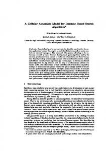
not be efficient to produce evenly distributed partitions in terms of workload of sub cell spaces. For example, in a cell space representing urban areas, urbanized cells might be concentrated in one part of the whole space, but sparse in other parts. Also, there might be some area excluded from urban sprawl (oceans, national parks, rough landscape, etc) over the space. But a Geo-CA model that simulates urban growth, e.g., SLEUTH, only evaluates those non-urbanized cells in non-exclusion areas. If the cell space was split into sub cell spaces evenly, and each computing unit was assigned only one sub cell space, then there would be a chance that some computing units have a large number of cells to process while others only have a few. To solve this workload inequality, a spatial-adaptive decomposition method has to be deployed. One approach is to decompose the cell space into uneven sub cell spaces according to the workload associated with them (Figure 3.2). Another approach is to reduce the granularity of decomposition, and to assign multiple sub cell spaces onto a computing unit in order to deliver approximately even workloads to computing units.
Figure 3.2 A spatial-adaptive decomposition: uneven parsing Another issue involved in the data decomposition is the neighborhood. The transition rules applied in a specific cell require its neighborhood’s data. While decomposing a cell space, every sub cell space has to include the neighboring cells of its “edge cells”. The “edge cells” refer to the edge cells of the cell space on which a corresponding computing unit actually applies the transition rule. To distinguish these “edge cells”, we call them “real edge cells”. In other words, a sub cell space assigned to a computing unit has overlapping belt(s) with its neighboring sub cell space(s). These overlapping belts are called “ghost cells”. A sub cell space’s ghost cells are actually the copies of the sub cell space’s neighboring sub cells space’s “real edge cells”. At the end of each transition process, the ghost cells have to be updated according to the new states of their origins which are owned by another computing unit, which creates communication overheads among computing units (Figure 3.3). In a Geo-CA model, not all the “real edge cells” change their states at each transition iteration. To minimize the
communication overheads, only those “ghost cells” whose origins’ states have been changed need to be updated. We call this approach “update on change”.
Figure 3.3 A cell space decomposition, a neighborhood pattern, and ghost cells’ updating
3.2.2 Process Decomposition and Hybrid Decomposition During the calibration processes, the evaluation process of a specific parameter combination is independent of the evaluation process of any other parameter combination. This characteristic perfectly fits the requirement of process decomposition. The latest version of SLEUTH uses the processdecomposition approach to shorten the computing time of the calibration processes. Each computing unit is assigned one or more parameter combination(s), or coefficient set(s), and the whole cell space, and performs simulations for preset Monte Carlo iterations (Figure 3.4). However, when dealing with a large dataset with a small number of parameter combinations, some computing units might be assigned massive workloads while others are idle. To solve this problem, one approach is to reduce the decomposition granularity. Instead of performing all the Monte Carlo iterations for a single parameter combination, each computing unit only perform one or more Monte Carlo iteration(s) for a parameter combination (Figure 3.5). Another approach is to combine data decomposition and process decomposition, and assign each computing unit sub cell space(s) and parameter combination(s) or Monte Carlo iteration(s) (Figure 3.6). By doing these, we are able to make sure that all the computing units can have almost evenly distributed workloads.
Figure 3.4 A coarse process decomposition
Figure 3.5 A fine process decomposition
Figure 3.6 A hybrid decomposition
3.2.3 Static Load-balancing and Dynamic Load-balancing In static load-balancing schema, data are completely decomposed and mapped to computing units before the computation starts. No adjustment will be made after that. It is suitable for regular and homogenous data. In contrast, in dynamic load-balancing schema, decomposition and mapping could be adjusted during the computation. Two main dynamic load-balancing approaches exist: the masterslaver model and the peer-to-peer model. In a master-slaver model, the data is partially decomposed and mapped by the master unit to slaver units before the initiation of the computation; during the computation, slaver units who finish processing their initial partitions request unprocessed partitions from the master until all the partitions are processed (Figure 3.7). In a peer-to-peer model, the data is completely decomposed and mapped among computing units; units who finish processing their own partitions request data from the nearest units that still have unprocessed data (Figure 3.8).
Figure 3.7 A master-slaver dynamic load-balancing
Figure 3.8 A peer-to-peer dynamic load-balancing Due to geo-spatial data’s irregularity and heterogeneous properties, and the various communication rates of parallel computing systems, dynamic load-balancing has the prospect to offer higher
performance, and more importantly, higher portability. However, dynamic load-balancing introduces more communication overhead than static load-balancing. Especially when a data decomposition method is used, large amounts of data have to be transferred among computing units. Thus, static loadbalancing might be more suitable for data decomposition. If a process decomposition method is deployed, dynamic load-balancing might be more efficient since only a little data, e.g., parameter combinations, Monte Carlo seeds, needs to be transferred among computing units.
4. Conclusions Cellular Automata models are powerful simulation tools in geographic research and applications. However, the rapidly increasing amount of geo-spatial and non-spatial data and high computational complexities make Geo-CA models, especially the calibration processes involved, extremely timeconsuming and sometimes infeasible in practice. This paper investigates the possibility of using parallel computing technologies to improve the performance of the calibration processes of Geo-CA models, and depicts some challenges and possible approaches to parallelize Geo-CA models. In conclusion, Geo-CA is very suitable for parallelization. But geo-spatial data’s irregularity and heterogeneous properties introduce some challenges to the decomposition and load-balancing processes. Spatial-adaptive data decomposition, update on change, small granularity process decomposition and hybrid decomposition should deliver better (or more even) workload distribution onto computing units. Static load-balancing should be more suitable when data decomposition methods are used, and dynamic load-balancing should be more efficient when process decomposition methods are used. High performance obtained by using parallel computing technologies enables the removal of simplifying assumptions and makes a comprehensive (full) calibration possible.
References: Clarke, K. C. (2003). "Geocomputation's Future at the Extremes: High Performance Computing and Nanoclients." Parallel Computing 29(10): 1281-1295. Clarke, K. C. and L. J. Gaydos (1998). "Loose-coupling a Cellular Automaton Model and GIS: Longterm Urban Growth Prediction for San Francisco and Washington/Baltimore." International Journal of Geographical Information Science 12(7): 699-714. Goldstein, N. C. (2003). Brains VS Braun – Comparative strategies for the calibration of a cellular automata-based urban growth model. 7th International Conference on GeoComputation, Southampton, England. Grama, A., A. Gupta, et al. (2003). Introduction to Parallel Computing. New York, Addison-Wesley.
Guan, Q., L. Wang, et al. (2005). "An Artificial-Neural-Network-based, Constrained CA Model for Simulating Urban Growth." Cartography and Geographic Information Science 32(4): 369 - 380. Li, X. and A. G. O. Yeh (2002). "Neural-network-based Cellular Automata for Simulating Multiple Land Use Changes Using GIS." International Journal of Geographical Information Science 16(4): 323343. Silva, E. A. and K. C. Clarke (2002). "Calibration of the SLEUTH Urban Growth Model for Lisbon and Porto." Computers, Environment and Urban Systems 26: 525–552. White, R. and G. Engelen (1994). "Cellular Dynamics and GIS: Modeling Spatial Complexity." Geographical Systems 1: 237-253. Wu, F. and C. J. Webster (1998). "Simulation of Land Development through the Integration of Cellular Automata and Multi-criteria Evaluation." Environment and Planning B 25: 103-126.