A Machine Learning Framework for Stock Selection

A Machine Learning Framework for Stock Selection XingYu Fu∗†‡ ,JinHong Du‡ ,YiFeng Guo‡ ,MingWen Liu∗† ,Tao Dong‡ ,XiuWen Duan‡ ∗ Likelihood

Technology Private Fund ‡ Sun Yat-sen University

† ShiningMidas

arXiv:1806.01743v2 [q-fin.PM] 8 Aug 2018

{f uxy28, dujh7, guoyf 9, dongt5, duanxw3}@mail2.sysu.edu.cn maxwell@alphaf uture.cn

Abstract—This paper demonstrates how to apply machine learning algorithms to distinguish “good” stocks from the “bad” stocks. To this end, we construct 244 technical and fundamental features to characterize each stock, and label stocks according to their ranking with respect to the return-to-volatility ratio. Algorithms ranging from traditional statistical learning methods to recently popular deep learning method, e.g. Logistic Regression (LR), Random Forest (RF), Deep Neural Network (DNN), and the Stacking, are trained to solve the classification task. Genetic Algorithm (GA) is also used to implement feature selection. The effectiveness of the stock selection strategy is validated in Chinese stock market in both statistical and practical aspects, showing that: 1) Stacking outperforms other models reaching an AUC score of 0.972; 2) Genetic Algorithm picks a subset of 114 features and the prediction performances of all models remain almost unchanged after the selection procedure, which suggests some features are indeed redundant; 3) LR and DNN are radical models; RF is risk-neutral model; Stacking is somewhere between DNN and RF. 4) The portfolios constructed by our models outperform market average in back tests. Index Terms—Quantitative Finance; Stock Selection; Machine Learning; Deep Learning; Feature Selection;

I. I NTRODUCTION There are mainly three types of trading strategies to construct in financial machine learning industry, i.e. asset selection [1], which selects potentially most profitable assets to invest, portfolio management [2], which distributes fund into the assets to optimize the risk-profit profile, and timing [3], which determines the apposite time to enter or leave the market. Effective asset selection is the bedrock of the whole trading system, without which the investment will be an irreparable disaster even if the most advanced portfolio management and timing strategies are deployed, and we therefore focus on asset selection, to be more specific, stock selection problem, in this article. The essence of stock selection is to distinguish the “good” stocks from the “bad” stocks, which lies into the scenario of classification problem. To implement the classification system, some natural questions emerge: 1) how to label stock instances correctly? 2) what machine learning algorithms shall we choose? 3) what features to consider and how to select the best subset of features? 4) how to evaluate models’ performances? For question 1), we rank stocks according to the return-tovolatility ratio and label the top and bottom Q percent stocks as positive and negative respectively [5]. The stocks ranking

in the middle of all candidates are discarded. This labeling technique enjoys two major advantages: Firstly, profitability and risk are both taken into account to give a comprehensive measure of stocks’ performances, which is exactly the basic idea of Sharpe Ratio [15]; Secondly, only the stocks whose behaviors are archetypical are used to train the classifiers, by which the ambiguous noisy information is filtered out. For question 2), we train learning algorithms ranging from traditional statistical learning methods to recently popular deep learning method, e.g. Logistic Regression (LR) [11], Random Forest (RF) [10], Deep Neural Network (DNN) [14], and the Stacking [12], to solve the classification task. The Stacking architecture we used is a two-dimensional LR model whose inputs are the outputs of trained RF and DNN. By Stacking, we pack heterogeneous machine learning models into a single ensemble model which outperforms its every individual component. Further note that financial time series data is nonstationary and its signal-noise ratio is low, which engender the over-fitting problem [4], especially for DNN. Hence, state-ofthe-art mechanisms such as Dropout [8], Batch-Normalization [9] and Model Regularization [14] are applied to DNN to alleviate the issue. For question 3), 244 technical and fundamental features are constructed to characterize each stock while some of the features may be redundant which introduce noise and increase the computational burden, and therefore effective features subset selection is crucial. In this work, we apply the Genetic Algorithm (GA) [7] to conduct globally optimal subset searching in a search space with exponential cardinality, which outperforms random selection greatly in our experiments. For question 4), the effectiveness of selection strategy is validated in Chinese stock market in both statistical and practical aspects. We first use the traditional train-test evaluation to examine the prediction performance of our models. Then we use the outputs of models to construct portfolios to trade in real historical market competing with the market average. The evaluation result shows that: 1) Stacking of RF and DNN outperforms other models reaching an AUC score of 0.972; 2) GA picks a subset of 114 features and the prediction performances of all models remain almost unchanged after the selection procedure, which suggests some features are indeed redundant. 3) LR and DNN are radical investment models; RF is risk-neutral model; Stacking’s risk profile is somewhere

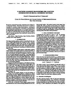
between DNN and RF. 4) The portfolios constructed by our models outperform market average in back tests. The implementation1 of the proposed stock selection strategy is available at Github and a data sample is also shared. II. DATASET C ONSTRUCTION A. Tail and Head Label Say there are M stock candidates and T days historical stock data. We use feature vector Xi (t) ∈ Rn to characterize the behavior of the ith stock up to the tth trading day and assign the return-to-volatility ratio yi (t, f ) to Xi (t) assessing the performance of the ith stock during trading period [t + 1, t + f ], where f is the length of the forward window. For each t under consideration, we obtain a set of feature vectors {Xi (t)|i ∈ {1, 2..., M }} and a set of return-tovolatility ratios {yi (t, f )|i ∈ {1, 2, ..., M }}. We rank stocks with respect to their return-to-volatility ratios and then do the following manipulations: • Label the top Q percent as positive, i.e. yi (t, f ) := 1; • Label the bottom Q percent as negative, i.e. yi (t, f ) := 0; • Discard the samples in the middle.

B. Initialization Suppose that the population size is 100. We initialize the 0th generation by randomly generating 100 binary vectors independently identically distributed with Binomial(244, 0.5). For each individual, we need to check if the sum of its chromosome’s components is not less than 1 to ensure the subset it represents is not empty. If the condition doesn’t hold, we need to regenerate this individual. C. Fitness To assess how good an individual is, we need to assign fitness to each individual. An individual is defined to be superior to the other if its fitness is bigger. In our work, we define the fitness of an individual as the AUC score of a machine learning model trained on the corresponding features subset. To be specific, for each individual, we use its chromosome to obtain a features subset and we train a logistic regression model on the training dataset only considering the corresponding features subset. Then we evaluate the LR model on the testing set and get the AUC value, which is set to be the fitness of the individual. D. Selection

Fig. 1. Data Split 2QT M To avoid data overlapping, at most b 100(1+f ) c samples can be labeled. Fig. 1. shows how to split data.

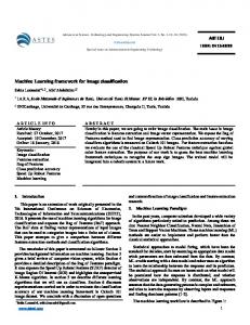
B. Feature Vector We construct 244 fundamental and technical features to characterize each stock at different trading days. Appendix lists the name of the constructed features. III. G ENETIC A LGORITHM BASED F EATURE S ELECTION Genetic Algorithm (GA) is a metaheuristic inspired by Darwin Natural Selection, where a population of individuals, representing a collection of candidate solutions to an optimization problem, are evolved towards better results through iteration. Each individual is assigned with a chromosome which can be mutated or crossed. The pipeline of GA is given by Fig. 2. A. Chromosome In this work, each individual’s chromosome is an encoding of a subset of features. Specifically, each individual’s chromosome is vector C ∈ {0, 1}n , such that C’s ith component: 1 if the ith feature is selected Ci := (1) 0 else where n denotes the total number of features, which is 244 in our case. 1 https://github.com/fxy96/Stock-Selection-a-Framework

After the computation of finesses, we can construct a probability distribution over the population by normalizing all individuals’ fitnesses and we select elites with respect to the distribution. Specifically, we randomly sample 100 individuals from the current population with replacement to form the next generation. The individuals with bigger fitnesses have bigger opportunities to be picked out. E. Crossover For each pair of sampled individuals obtained from the previous selection procedure, with probability 0.2 we implement the crossover mechanism, i.e. we randomly select a position on chromosome and exchange the genes of the two individuals at this position. F. Mutation After crossover, for each sampled individuals, with probability 0.1 we carry out the mutation procedure, i.e. we randomly select a component on this individual’s chromosome and alter its value. G. Evolution In each iteration, we repeat the above manipulations and record the best individual. Generally, the average fitness of the population will become increasing better as the iteration goes on and this is the reason why we call GA as evolutionary process. After 100 iterations, we terminate the evolution and selects the best individual as the best features subset representation.

Hyperparameter Initial Learning Rate Learning Rate Decay Rate Training Epochs Momentum Coefficient

Value 10−2 10−6 20 0.9

TABLE I LR H YPERPARAMETERS

forest are trained on different bootstrapping samples of training dataset and focus on different random feature subsets to break model correlation. It is proven, by both industry and academia, that RF can effectively decrease variance of model without increasing bias, i.e. conquers over-fitting problem, and therefore RF is a promising predictive method in finance machine learning industry, where over-fitting is a common problem. Table 2 shows the hyperparameters of RF. Hyperparameter Number of Trees Maximal Tree Depth Minimal Samples Number of Split Minimal Impurity of Split

Value 100 4 2 10−7

TABLE II RF H YPERPARAMETERS Fig. 2. Pipeline of GA

C. Deep Neural Network

IV. P REDICTIVE M ODELS In this section, we will discuss the details of models we use in our work, which are: Logistic Regression (LR), Random Forest (RF), Deep Neural Network (DNN), and the Stacking of RF and DNN. A. Logistic Regression LR is a classical statistical learning algorithm, which models the conditional probability of positive sample given the feature vector using the logistic function, i.e. P {Y = 1|X = x} = σ(β · x + b)

(2)

, where σ(t) = 1+e1 −t is the logistic function and β ∈ Rn , b ∈ R are the linear coefficients. The key to implement LR is to estimate the linear coefficients from historical labeled data, where in this paper, we apply the Stochastic Gradient Descent (SGD) with Nesterov momentum and learning rate decay [16] algorithm to minimize the log-likelihood loss function to this purpose. Although LR is a rather simple model, which results in relatively poor predictive ability, yet it is extensively used in financial machine learning industry since it is unlikely to suffer from over-fitting. Table 1 shows the hyperparameters of LR.

DNN, a technique that recently witnessed tremendous success in various tasks such as computer vision, speech recognition and gaming [17,18,19], is a potential power predictor in financial application. While DNN is prone to be stuck in poor local optimum if the training environment is highly noisy, and therefore effective mechanisms preventing over-fitting must be deployed if we want to use DNN in financial market. In this work, we implement a three-layer neural network to classify stocks, where Dropout, Batch-Normalization and L2 Regularization are used to avoid over-fitting. Its training is done through SGD with Nesterov momentum and learning rate decay. For most cases, the network converges after 20 epochs. Table 3 and Table 4 demonstrate network architecture and hyperparameters respectively. Layer Input Tensor Fully Connected Layer with L2 Regularizer ReLu Activation Dropout Layer Fully Connected Layer with L2 Regularizer ReLu Activation Batch-Normalization Layer Fully Connected Layer with L2 Regularizer Softmax Activation

B. Random Forest RF is a state-of-the-art machine learning technique that trains a collection of decision trees and makes classification prediction by averaging the output of each tree. The trees in

TABLE III N ETWORK S TRUCTION

Shape 128 × n c 128 × b n 2 128 × b n c 2 128 × b n c 2 128 × b n c 4 128 × b n c 4 128 × b n c 4 128 × 2 128 × 2

Hyperparameter Dropout Rate L2 Penalty Coefficient Momentum Coefficient Initial Learning Rate Learning Rate Decay Rate Training Epochs

Value 0.5 0.01 0.9 10−3 10−6 20

TABLE IV N ETWORK H YPERPARAMETERS

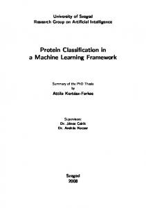
D. Stacking of RF and DNN Stacking is a technique to ensemble multiple learning algorithms, where a meta-level algorithm is trained to make a final prediction using the outputs of based-level algorithms as features. Generally, the stacking model will outperform its each based-level model due to its smoothing nature and ability to credit the classifiers which perform well and discredit those which predict badly. Theoretically, stacking is most effective if its based-level algorithms are uncorrelated. In this work, RF and DNN are used as based-level classifiers and LR is selected as meta-level algorithm. We first partition the original training dataset into three disjoint sets, named as Train-1, Train-2, and Validation. Train-1 and Train-2 serve as the training set of based-level classifiers, in which the DNN is trained on the concatenation of Train-1 and Train-2 and RF is trained solely on Train-2. By training like this, the two based-level algorithms’ behaviors will be significantly uncorrelated , which is the prerequisite for a well-performed stacking, for two reasons: 1) RF and DNN belong to, in nature, two utterly different types of algorithms; 2) DNN is trained in a ”Fore-Sighted” way while RF is trained in a ”Short-Sighted” way. Validation is then used to train the meta-level LR model, where the inputs to LR is the predictions from trained-DNN and trained-RF on the Validation. The pipeline of training our stacking model is shown in Fig. 3..

A. Statistical Analysis Table 5 and Table 6 demonstrate the statistical indexes of different models before and after GA feature selection. The training dataset is constructed from Chinese stock data ranging from 2012.08.08 to 2013.02.01 and the testing dataset is constructed from 2013.02.04 to 2013.03.08. Fig. 4. shows the pipeline of our statistical evaluation procedure. AUC Accuracy Precision Recall F1 TPR FPR

LR 0.964 0.903 0.871 0.945 0.907 0.945 0.139

RF 0.965 0.918 0.916 0.922 0.919 0.922 0.084

DNN 0.970 0.913 0.875 0.963 0.917 0.963 0.138

Stack 0.972 0.919 0.904 0.938 0.921 0.938 0.099

TABLE V S TATISTICAL I NDEXES BEFORE F EATURE S ELECTION

AUC Accuracy Precision Recall F1 TPR FPR

LR 0.966 0.908 0.886 0.936 0.911 0.936 0.119

RF 0.970 0.918 0.919 0.916 0.918 0.916 0.079

DNN 0.958 0.869 0.819 0.946 0.878 0.946 0.207

Stack 0.973 0.927 0.919 0.936 0.928 0.936 0.081

TABLE VI S TATISTICAL I NDEXES AFTER F EATURE S ELECTION

Fig. 3. Pipeline of Training Stacking

V. R ESULT P RESENTATION AND E MPIRICAL A NALYSIS In this section, we present our result and analyze it from both statistical aspect and practical (portfolio management) aspect.

Fig. 4. Pipeline of Statistical Evaluation

As we can see from Table 5 and Table 6:

•

•

•

Stacking of DNN and RF outperforms other models before and after feature selection reaching the highest AUC score, which shows the promising prospect of ensemble learning in financial market. All the statistical indexes remain almost unchanged before and after feature selection, which shows some features are indeed redundant. For both LR and DNN models, their Recall scores are notably higher than their Precision scores, which indicates, in plain English, LR and DNN are radical investment models. While for RF, its Recall score is commensurate to its Precision score, suggesting that RF is more likely to be a risk-neutral investment model. As for Stacking, it’s risk profile is somewhere between RF and DNN since it is a combination of RF and DNN.

B. Portfolio Analysis There is a setback of our statistical evaluation procedure, i.e. only the stocks in the Q percent tail and head are included in the test sets, which means we only test our model in the unequivocal test samples. Therefore, a more close-to-reality evaluation is needed. To this end, for each model, we use its output, which is a vector of scalers ranging from zero to one, to construct portfolio and trade it in historical market competing with the market average. Fig. 5., Fig. 6., and Fig. 7. demonstrate the back test results showing that our stock selection strategy can construct profitable portfolios conquering the market average.

Fig. 5. Portfolio Management starts from 2015.11.30



ACKNOWLEDGMENT We would like to say thanks to YuYan Shi, ZiYi Yang, MingDi Zheng, and Yuan Zeng for their incipient involvement of the project. We also thank Professor ZhiHong Huang of Sun Yat-sen University for his patient and generous help throughout the research. R EFERENCES [1] Van der Hart J, Slagter E, Van Dijk D. Stock selection strategies in emerging markets[J]. Journal of Empirical Finance, 2003, 10(1-2): 105132. [2] Sharpe W F, Sharpe W F. Portfolio theory and capital markets[M]. New York: McGraw-Hill, 1970. [3] Shen P. Market-timing strategies that worked[J]. 2002. [4] Lopez de Prado M. The 10 Reasons Most Machine Learning Funds Fail[J]. 2018. [5] Huerta R, Corbacho F, Elkan C. Nonlinear support vector machines can systematically identify stocks with high and low future returns[J]. Algorithmic Finance, 2013, 2(1): 45-58. [6] Pai P F, Lin C S. A hybrid ARIMA and support vector machines model in stock price forecasting[J]. Omega, 2005, 33(6): 497-505. [7] Yang J, Honavar V. Feature subset selection using a genetic algorithm[M]//Feature extraction, construction and selection. Springer, Boston, MA, 1998: 117-136. [8] Srivastava N, Hinton G, Krizhevsky A, et al. Dropout: A simple way to prevent neural networks from overfitting[J]. The Journal of Machine Learning Research, 2014, 15(1): 1929-1958. [9] Ioffe S, Szegedy C. Batch normalization: Accelerating deep network training by reducing internal covariate shift[J]. arXiv preprint arXiv:1502.03167, 2015. [10] Liaw A, Wiener M. Classification and regression by randomForest[J]. R news, 2002, 2(3): 18-22. [11] Harrell F E. Ordinal logistic regression[M]//Regression modeling strategies. Springer, New York, NY, 2001: 331-343. [12] Deroski S, enko B. Is combining classifiers with stacking better than selecting the best one?[J]. Machine learning, 2004, 54(3): 255-273. [13] Bradley A P. The use of the area under the ROC curve in the evaluation of machine learning algorithms[J]. Pattern recognition, 1997, 30(7): 11451159. [14] Goodfellow I, Bengio Y, Courville A, et al. Deep learning[M]. Cambridge: MIT press, 2016. [15] Sharpe W F. The sharpe ratio[J]. Journal of portfolio management, 1994, 21(1): 49-58. [16] Ruder S. An overview of gradient descent optimization algorithms[J]. arXiv preprint arXiv:1609.04747, 2016. [17] Krizhevsky A, Sutskever I, Hinton G E. Imagenet classification with deep convolutional neural networks[C]//Advances in neural information processing systems. 2012: 1097-1105. [18] Hannun A, Case C, Casper J, et al. Deep speech: Scaling up end-to-end speech recognition[J]. arXiv preprint arXiv:1412.5567, 2014. [19] Silver D, Schrittwieser J, Simonyan K, et al. Mastering the game of go without human knowledge[J]. Nature, 2017, 550(7676): 354.

A PPENDIX

AccountsPayablesTDays AdminiExpenseRate ARTRate BLEV CashRateOfSales CMRA CTP5 CurrentAssetsTRate DAVOL10 DAVOL5 DDNCR DebtEquityRatio DHILO DVRAT EGRO EMA120 EMA5 EPS EquityToAsset ETOP FinancialExpenseRate FixAssetRatio GrossIncomeRatio HSIGMA InventoryTDays InvestCashGrowRate LFLO LongDebtToWorkingCapital MA10 MA20 MA60 MFI NetAssetGrowRate NetProfitRatio NonCurrentAssetsRatio NPToTOR OperatingProfitGrowRate OperatingProfitToTOR OperCashGrowRate PB PE PSY REVS10 REVS5 ROA5 ROE5 RSTR12 SalesCostRatio SUE TOBT TotalAssetsTRate TotalProfitGrowRate VOL120 VOL240 VOL60 REC GREC DAREV SFY12P GSREV FSALESG

AccountsPayablesTRate ARTDays ASSI BondsPayableToAsset CashToCurrentLiability CTOP CurrentAssetsRatio CurrentRatio DAVOL20 DDNBT DDNSR DebtsAssetRatio DilutedEPS EBITToTOR EMA10 EMA20 EMA60 EquityFixedAssetRatio EquityTRate ETP5 FinancingCashGrowRate FixedAssetsTRate HBETA IntangibleAssetRatio InventoryTRate LCAP LongDebtToAsset LongTermDebtToAsset MA120 MA5 MAWVAD MLEV NetProfitGrowRate NOCFToOperatingNI NPParentCompanyGrowRate OperatingExpenseRate OperatingProfitRatio OperatingRevenueGrowRate OperCashInToCurrentLiability PCF PS QuickRatio REVS20 ROA ROE RSI RSTR24 SaleServiceCashToOR TaxRatio TotalAssetGrowRate TotalProfitCostRatio VOL10 VOL20 VOL5 WVAD DAREC FY12P GREV DASREV FEARNG TA2EV

AdminiExpenseRate ARTRate BLEV CashRateOfSales CMRA CTP5 CurrentAssetsTRate DAVOL10 DAVOL5 DDNCR DebtEquityRatio DHILO DVRAT EGRO EMA120 EMA5 EPS EquityToAsset ETOP FinancialExpenseRate FixAssetRatio GrossIncomeRatio HSIGMA InventoryTDays InvestCashGrowRate LFLO LongDebtToWorkingCapital MA10 MA20 MA60 MFI NetAssetGrowRate NetProfitRatio NonCurrentAssetsRatio NPToTOR OperatingProfitGrowRate OperatingProfitToTOR OperCashGrowRate PB PE PSY REVS10 REVS5 ROA5 ROE5 RSTR12 SalesCostRatio SUE TOBT TotalAssetsTRate TotalProfitGrowRate VOL120 VOL240 VOL60 REC GREC DAREV SFY12P GSREV FSALESG CFO2EV

ARTDays ASSI BondsPayableToAsset CashToCurrentLiability CTOP CurrentAssetsRatio CurrentRatio DAVOL20 DDNBT DDNSR DebtsAssetRatio DilutedEPS EBITToTOR EMA10 EMA20 EMA60 EquityFixedAssetRatio EquityTRate ETP5 FinancingCashGrowRate FixedAssetsTRate HBETA IntangibleAssetRatio InventoryTRate LCAP LongDebtToAsset LongTermDebtToAsset MA120 MA5 MAWVAD MLEV NetProfitGrowRate NOCFToOperatingNI NPParentCompanyGrowRate OperatingExpenseRate OperatingProfitRatio OperatingRevenueGrowRate OperCashInToCurrentLiability PCF PS QuickRatio REVS20 ROA ROE RSI RSTR24 SaleServiceCashToOR TaxRatio TotalAssetGrowRate TotalProfitCostRatio VOL10 VOL20 VOL5 WVAD DAREC FY12P GREV DASREV FEARNG TA2EV ACCA