A MAD APPROACH FOR SOLVING PART-SELECTION ... - CiteSeerX

APPEARS IN THE PROCEEDINGS OF AI IN DESIGN, 1998. DO NOT COPY OR DISTRIBUTE THIS VERSION OF THE PAPER

A MAD APPROACH PROBLEMS

FOR

SOLVING

PART-SELECTION

TIMOTHY P. DARR1, WILLIAM P. BIRMINGHAM The University of Michigan Electrical Engineering and Computer Science Department Ann Arbor, Michigan, 48109 USA AND NANCY SCALA

Abstract. Part selection is a fundamental problem in engineering design where off-the-shelf components are selected and assembled into an artifact that meets a designer's specifications. Part selection is a combinatorial search problem that has both practical applications for design and general importance to AI by providing insight on solving tough search problems. We construct a mapping from constraintsatisfaction problems, which have well-known techniques for mitigating combinatorial problems, to part selection. Through this mapping we have identified and present in this paper: general conditions for backtrack-free search for a class of CSPs that apply directly to part-selection problems; a heuristic for reducing search based on the structure of a variable’s domain; and, an efficient algorithm for preprocessing constraint graphs. We also present experimental results illustrating the efficiency of our methods.

1. Introduction Part selection is a fundamental problem in engineering design where off-theshelf components are selected and assembled into an artifact that meets a designer's specifications. Part selection is a combinatorial search problem that has both practical applications for design and general importance to AI by providing insight on solving tough search problems. This paper presents a

1

Now at Trilogy Development Group, Austin, TX.

2

T.P. DARR, W.P. BIRMINGHAM, N. SCALA

computational model, and set of heuristics, for modeling and solving partselection problems. In general, a part-selection problem is exponentially complex due to three factors: (1) many parts may be selected to implement each of the required functions of the artifact, (2) parts can implement more than one function (the multi-function part problem) (Haworth, Birmingham and Haworth 1993) or a set of parts may be needed to implement a single function, and (3) parts often require additional, “support” functions to operate correctly (Mittal and Falkenhainer 1990), which leads to the horizon effect. In addition, the solution must satisfy constraints and preferences. Thus, as a practical matter, it is critical that search techniques be developed to manage the problem complexity. Design researchers often manage complexity using domain-specific rules. This approach is effective and has advantages, but its weakness is that it does not apply across domains (i.e., different design problems). In addition, domain-independent techniques exist to manage the complexity of partselection problems based on properties of the constraints, parts, and catalogs themselves. In this paper, we present a computational model for part-selection problems based on a specialization of the constraint-satisfaction problem (CSP). The CSP literature includes a number of domain-independent methods that may reduce search complexity under certain circumstances. Thus, we can exploit the many useful results for solving CSPs for part selection. A part-selection problem can potentially be made tractable by taking advantage of these results. We construct a mapping from CSPs to part selection, and through this mapping we have identified: general conditions for backtrack-free search for a class of CSPs that apply directly to part-selection problems; a heuristic for reducing search based on the structure of a variable’s domain; and, an efficient algorithm for preprocessing constraint graphs (Darr 1997). In this paper, we first introduce the multi-attribute domain CSP (MADCSP), which is a specialization of the traditional CSP that has properties that are very useful for solving part-selection and other problems, including the conditions for backtrack-free search. We then formally define the partselection problem, and map it into the MAD-CSP formalism. Finally, we present some experimental results and conclude the paper.

2. Multi-Attribute Domain CSPs The traditional CSP model can be awkward when the domain values are multiattribute; that is when each domain element is described as a tuple of values. Part selection is an example of a problem where the domains (i.e., parts) are multi-valued (Darr 1997). The multi-attribute domain CSP is a convenient and natural way to represent these problems.

3

A MAD APPROACH FOR SOLVING PART-SELECTION PROBLEMS

2.1.1 MAD-CSP DEFINITION The notation for multi-attribute domain variables is illustrated in TABLE 1 for variable vi. The first column, labeled “Variable vi”, lists the domain elements for each variable. The value of a domain element is the tuple shown as the rows in the table listed under the columns labeled “Domain Attribute ai1, ai2, ..., aiν”.2 Each αi,kρ is the value of the ρ-th domain attribute of the k-th domain element. The shaded regions in the table are the values of the domain elements. Constraints are defined over domain attributes, rather than variables as in single-attribute CSPs. TABLE 1: Multi-Attribute Domain Variable Notation

Variable vi υi,1 υi,2 ... υi,d

ai1 αi,11 αi,21 αi,d1

Domain Attribute ai2 ... aiν ... αi,12 αi,1ν 2 ... αi,2 αi,2ν ... ... αi,d2 αi,dν

TABLE 1 helps to illustrate why traditional CSPs are awkward for multiattribute problems. For a traditional CSP, each domain attribute would become a variable. To maintain proper correspondences among the domainattribute values as required by the problem, constraints would be needed to link values across these variables, so that as a domain value is assigned to a variable, the corresponding value in other variables would also be assigned. For example, if ai1 and ai2 were variables, then a constraint would be required between the values αi,11 and αi,12, the values αi,21 and αi,22, and so forth, so that if αi,11 is assigned to ai1, then αi,12 is assigned to ai2. Thus, the size of the network in terms of both variables and constraints would be greatly increased. As time and space required to solve a CSP is exponentially proportional to the number of variables, and (at least) linearly related to the number of constraints, reducing the number of both of these can be beneficial. Of course, there are cases where this representation affords no effective relief from problem combinatorics. The multi-attribute domain constraint-satisfaction problem (MAD CSP) is defined as follows: •

a set of variables V={v1, ..., vi, ..., vn}. •

2

The precondition evaluation function, vipre defines when a value is to be selected for the variable. If the precondition is true, then the variable is active; otherwise it is inactive (Mittal and Falkenhainer 1990).

A superscript is used to distinguish domain attributes from domain elements.

4

3

T.P. DARR, W.P. BIRMINGHAM, N. SCALA

•

a set of domain attributes for each variable Ai = (column labels in TABLE 1).

•

a set of discrete multi-attribute domain elements for each variable, vi = {υi,1, ..., υi,d} (row labels in TABLE 1). •

the value of each domain element υi,k is given by a tuple of domain-attribute values: υi,k = (row entries in TABLE 1), where αi,kρ is the value of domain attribute aiρ for domain element υi,k. A domain is “ordered” when its values are ordered by the ≤ relation.

•

For variables with ordered attributes, an interval domain representation can be used, vi = , where aiρ = [αiρ, ωiρ], such that ∀αi,kρ, αiρ ≤ αi,kρ ≤ ωiρ. This representation is key for the properties and heuristics that will be presented later.

•

a value function that assigns a utility value to each domain element u(υi,k) = Σρ wρ * αi,k ρ with Σ ρ w ρ = 1.3

•

a set of constraints, C = {c1, ..., cj, ..., cm}, that restrict the allowed assignments to domain attributes. Constraints are defined over a subset of all domain attributes, Aj, known as the constraint’s arguments. •

Each assignment A* ∈ cj satisfies the constraint (it is feasible); all other assignments violate the constraint (they are infeasible).

•

The constraint-evaluation function gj defines when the constraint is satisfied. If the function evaluates to true, then the constraint is satisfied; otherwise, it is violated.

•

Constraint-propagation functions hj(akr) restrict the domain of argument akρ, given the possible assignment of domain values to all other arguments.

•

The precondition evaluation function, cjpre, defines when a constraint cj is active. If the precondition is true, the constraint is active; otherwise it is inactive (Mittal and Falkenhainer 1990).

•

The constraint network is a graph G = (V, C).

•

A solution to a CSP is an assignment of values to variables such that all constraints are satisfied.

The attribute values are normalized before the value function is evaluated.

5

A MAD APPROACH FOR SOLVING PART-SELECTION PROBLEMS

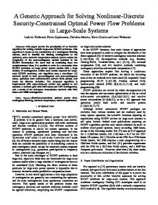
Figure 1 shows an example multi-attribute CSP, with three variables and four constraints. The first variable is defined by two domain attributes (a11, a12), and the latter two variables are defined by three domain attributes (a21, a22, a23 and a31, a32, a33, respectively). Most of the attributes in this example are ordered, so the interval representation, aiρ = [αiρ, ωiρ] applies. Attibute a23, however, is a set {cable5, cable9}, so the interval representation does not apply. v

1

υ1 , 1 υ1 , 2 υ1 , 3

a 11

a 12

v

1

2

2

1

5

4

υ2 , 1 υ2 , 2 υ2 , 3

v

3

υ3 , 1 υ3 , 2

2

a 21

a 22

a 23

3

4

c able 9

6

7

c able 5

7

1

c able 9

a 31

a 32

a 33

1

2

5

4

3

4

Constraints c1: a11 Š a22 c2: a12 + a22 + a33 Š 12 c3: a21 Š 2 * a32 c4: a21 = cable9 Figure 1. Example Multi-Attribute Domain CSP

2.2. PROPERTIES This section defines properties of the multi-attribute domain CSP, which follow from related work in single attribute-domain interval CSPs. 2.2.1. Consistency A variety of preprocessing consistency techniques based on CSP network properties efficiently remove infeasible domain elements, thereby reducing the search space. An efficient technique that achieves a level of consistency requiring only local reasoning is 2-consistency (or arc-consistency for binary constraint graphs). A constraint whose precondition is true is 2-consistent if for each attribute in the constraint's arguments and every assignment to that attribute, there exist values for all the other attributes in the constraint's arguments that satisfy the constraint (Freuder 1978; Mackworth 1977). If a constraint is consistent, then each value of each attribute in the constraint’s arguments is a consistent value. (Note: we define consistency over attributes, not variable domains.) The propagation function hjconsistent(akρ) yields a set of consistent values for the attribute akρ. The predicate consistent(cj) is true if cj is consistent; the

6

T.P. DARR, W.P. BIRMINGHAM, N. SCALA

predicate consistent(vi) is true if consistent(cj) for every cj that includes a domain attribute of vi in its arguments. When applied to part selection, consistency reduces the problem size by removing infeasible parts from further consideration (this is shown below). For a certain class of problems with monotone constraints, only the minimum and maximum domain values of a variable need to be checked for consistency, improving the efficiency of consistency algorithms (Van Hentenryck, Deville and Teng 1992). This has been used in constraint-logic programming systems by representing the domain as an interval and evaluating constraints using interval arithmetic, since interval arithmetic only uses the interval bounds to evaluate an expression (Van Hentenryck, Simonis and Dincbas 1992). In the cases where the interval representation of Section 2.1.1 applies and the constraints are monotone, we need only check endpoints (the bounds of the interval) to achieve consistency. Thus, we exploit optimal time complexity algorithms, where arc consistency can be found in linear time with respect to the number of constraints (Darr 1997). 2.2.2. Decomposability Decomposability, or n-consistency, is a stronger property than consistency. Decomposability means that any combination of domain values satisfies all the constraints (Freuder 1978; van Beek 1992). The predicate decomposable(cj) is true if cj is decomposable; the predicate decomposable(vi) is true if decomposable(cj) for every cj that includes a domain attribute of vi in its arguments. Decomposability is the ultimate goal of any CSP solver. 2.2.3. Monotonicity Monotonicity is a key element for the properties and heuristics that follow. A constraint is monotone decreasing in aiρ if an assignment that includes αi,kρ satisfies the constraint, then any assignment that includes αi,mρ for all αi,mρ < αi,kρ also satisfies the constraint. We define monotone increasing constraints in a similar way (Darr, 1997). A constraint is monotonic if for each attribute in the constraint's arguments, the constraint is monotone increasing or monotone decreasing, or both, in that attribute. If a constraint is monotone increasing or decreasing in attribute aiρ, then interval versions of the constraint propagation functions are defined (hjconsistent(aiρ)). These functions return a consistent interval, instead of a set of consistent values. Figure 2 shows the monotonicities for the example multiattribute domain CSP of Figure 1

7

A MAD APPROACH FOR SOLVING PART-SELECTION PROBLEMS

attribute a11 a12 a21 a22 a31 a32 a33

monotonicity decreasing decreasing increasing decreasing increasing decreasing

constraint c1, c2 c3 c1 c2 c3 c2

Figure 2. Example Problem Monotonicities

2.2.4. Boundary-Element A domain element is a boundary element if it lies on the boundary of the interval representation of the domain, and is related to the problem constraints in a specific way. Let vi = , aiρ = [αiρ, ωiρ], be the interval representation for variable vi as defined in Section 2.1.1. Domain element υi,k is a boundary element if the following holds: •

αi,kρ = αiρ for all aiρ such that cj is monotone decreasing in aiρ, and

•

αi,kρ = ωiρ for all aiρ such that cj is monotone increasing in aiρ.

In Figure 1, domain element υ3,2 is a boundary element, since α3,22 = 3 (a32 is monotone increasing and a32 = [2 3]) and α3,23 = 4 (a33 is monotone decreasing and a33 = [4 5]). The boundary-element property requires that the domain attributes be ordered and the constraints be monotonic over the set of domain-attribute values (Darr 1997). Boundary elements are particularly important to partselection and configuration-design problems, since it provides a way to reduce the choices in a catalog to a single part, thereby reducing the search space. Section 2.4 uses the boundary part property to state the conditions for backtrack-free search. 2.3. DECOMPOSABILITY HEURISTIC There exist many methods for calculating consistent sets or intervals for a variable. Consistency does not, however, guarantee decomposability. Therefore, it is necessary to identify heuristics for achieving decomposability. This section presents an algorithm for one such heuristic that uses the monotonicity of constraints, and ordered domain-attribute values to partition the variable domains. Figure 3 shows the algorithm. The domain partitioning heuristic is based on the observation that for monotonic constraints, infeasible values are found at the interval endpoints, though these are not necessarily the only values that violate the constraints. Eliminating these elements, however, can sometimes dramatically reduce the search needed to achieve decomposability. We assume that the elements with the smallest and largest value of a domain attribute can

8

T.P. DARR, W.P. BIRMINGHAM, N. SCALA

be accessed using the functions min(vi, aiρ) and max(vi, aiρ), respectively. The following paragraphs describe the algorithm in more detail. vi = PartitionDomain(vi ) 1 1. vi = v i 2 2. vi = ∅ 3. for each ai ρ ∈ Ai 4. if aiρ_decreasing > 0 1 1 5. vi = v i - max(vi, aiρ) 2 2 6. vi = v i + max(vi , ai ρ) ρ 7. if ai _increasing > 0 1 1 8. vi = v i - min(vi, aiρ) 2 2 9. vi = v i + min(vi , ai ρ) 1 10. if vi = ∅ 11. create viπ using some ordering of domain values 12. store state(vi) and return 13. store state(vi) and return Figure 3. Partition Domain Algorithm

For bookkeeping purposes, a monotonicity counter is kept, for each domain attribute aiρ. This counter records the number of constraints that are monotone increasing in aiρ (aiρ_increasing), and monotone decreasing in aiρ (aiρ_decreasing). These counters record if the domain attribute is constrained by any constraint; if the counter is non-zero, then the domain attribute is constrained. As constraints become decomposable, the monotonicity counters are decremented, as appropriate. The Partition Domain algorithm creates a partition viπ = and initializes vi1 to vi and vi2 to the NULL set (lines 1-2). Partitions are created by removing elements from vi1 and adding them to vi2. For each domain attribute aiρ (line 3), if the monotonicity counter for monotone decreasing constraints is non-zero (line 4), meaning that there is a non-decomposed constraint that constrains the assignment to aiρ, the domain element with the greatest value for aiρ is removed from vi1 and added to vi2 (lines 5 and 6). A similar operation is performed for montone increasing constraints (lines 7-9). If the domain of vi1 becomes empty at any time, the heuristic fails, and an alternate heuristic is attempted (lines 10, 11). Once a partition is successfully created, the partition is stored for backtracking purposes in a state variable and the algorithm terminates (line 12). Thus, we are not guaranteed to find a decomposable network without backtracking using this heuristic. Details on the backtracking algorithm can be found elsewhere (Darr 1997). Figure 4 shows the result of applying the variable-domain partitioning heuristic for the example variable v2, shown in Figure 1: •

domain element υ2,2 is removed since it is constrained by constraint c2, a monotone decreasing constraint in a22, (see Figure 2) and υ2,2 has the highest value for a22.

9

A MAD APPROACH FOR SOLVING PART-SELECTION PROBLEMS

•

domain element υ2,3 is removed since it is constrained by constraint c1, a monotonicity increasing constraint in a22, (see Figure 2) and it is constrained by constraint c3, a monotone decreasing constraint in a21, (see Figure 2), and υ2,3 has the smallest and largest values for a22 and a21, respectively.

v2 υ2, 1 υ2, 2 υ2, 3 1

v2

a2

υ2, 1

3

a2

a21

a22

3 6 7

4 7 1

2

4

counter a2 _decreasing a22_increasing 2

1

v2

a2

υ2, 2 υ2, 3

6 7

a2

2

7 1

value 1 1

Figure 4. Example Variable-Domain Heuristic (v2)

2.4 BACKTRACK-FREE SEARCH In single attribute-domain CSPs, there exist several techniques and properties for backtrack-free search. The algorithm AC-5 has been shown to yield a backtrack-free assignment, without search, for binary CSPs with constraints of the form a*x = b*y + c, a*x = b*y + c or a*x = b*y + c. This is done by selecting the minimum value from each domain (Van Hentenryck, Deville and Teng 1992). This section extends the results to MAD-CSPs using the boundary-element property. Theorem 1 defines the backtrack-free conditions MAD-CSPs. We state without proof the theorem and corollary (see Darr (1997) for the proofs). Theorem 1: A multi-attribute domain CSP is backtrack-free if a boundary element exists for each vi ∈ V. Corollary 1.1: If υi,k is a boundary element, then vi = υi,k is a feasible assignment to vi, or no feasible assignment exists. An algorithm for assigning boundary elements to variables is a straightforward application of Corollary 1.1. This algorithm takes a variable as input and returns the updated variable as output. If there is a boundary element for that variable, then all non-boundary elements are removed, and the boundary element is returned as an assignment to the variable.

10

T.P. DARR, W.P. BIRMINGHAM, N. SCALA

3. Part Selection This section defines the part-selection problem, including definitions of: •

parts, catalogs, and designs,

•

constraints, and

• the problem specification. Part selection is solved by selecting pre-defined parts that can be combined only in certain ways to implement some high-level functionality. In other words, new parts cannot be created during the design process, constraints restrict the part combinations, and parts implement functions whose combination results in the desired user-specified functionality (Mittal and Frayman 1989). For our purposes, a function is a property of a part that, alone or in combination with other parts, achieves some user-defined functionality. The design is the collection of parts that implements the highlevel functionality, and meets other criteria as well, such as optimality. Attributes are used to describe parts. An attribute is a two-tuple , where ak is the attribute’s name and dk is its domain. The domain is the set of values that can be assigned to the attribute, and is restricted to scalar values. Parts are sets of attributes, part = {, ..., , , ..., }. A special subset of part attributes {, ..., } is the partfunction multiplicity (partpfm), which is the set of functions implemented by the part; the part implements fmk instances of fk (Haworth, Birmingham and Haworth 1993; Mittal and Frayman 1989). A catalog is a collection of parts, catalog = {parti: i = 1, ... D} generally organized in any fashion, though typically they are organized by vendor product line. The set of all catalogs is catalogs = {catalogi: i = 1, ..., M}. The catalog-function multiplicity, catalogpfm = {partipfm: i = 1, ..., D}, is the set of part-function multiplicities of all parts in the catalog. Figure 5 shows an example catalog. part name c1

cost 20.0

power 3.00

c2

21.0

2.90

c3 c4 i1 i2 t1

11.0 10.0 3.1 3.0 5.0

2.10 2.50 0.35 0.40 1.00

pfm , , , ,

Figure 5. Example Catalog

11

A MAD APPROACH FOR SOLVING PART-SELECTION PROBLEMS

Constraints are fundamental to the design process, since they restrict the allowed part combinations. Constraints define a network that describes the relationships among all the parts in the design. A constraint is a relation cj defined over a subset of the part attributes that restrict the attribute domains. The design problem specifies the functions to implement, the constraints to satisfy, the set of catalogs, and designer preferences over various designs, represented as a linear, weighted value function (Fishburn 1970). Formally, the design-problem is a tuple , that describes the desired design in terms of a set of specifications: •

required functions = {: fmk instances of fk are required} •

fkφ is the φ-th instance of fk (φ ∈ {1, ..., fmk})

•

constraints = ∪j cj, is the set of feasibility constraints,

•

catalogs = ∪i catalogi, is a set of part catalogs,

•

u() is a linear, weighted value function that assigns a real number to a design or part, defines a partial order on the designs or parts, and represents the desirability of the part or design from the designer’s perspective •

u(part) = Σk wk * v(ak), Σk wk = 1, ∈ part4

•

u(design) = Σk wk * v(ak), Σk wk = 1, ∈ part ∈ design

A solution to the design problem (a design) is a set of parts S with the following properties: •

For each fkφ ∈ required-functions, there exists a part ∈ S such that ∈ partpfm, for all part ∈ S

•

The set of parts satisfies all constraints.

•

The set of parts is optimal with regard to the user’s preferences, with perhaps some restrictions (such as locality).

3.1. MAPPING THE MAD-CSP TO PART SELECTION The part-selection problem maps naturally to the MAD-CSP; TABLE 2 shows the mapping. Preconditions are introduced into the part-selection problem to represent the dynamic nature of part-selection constraints. Consistency-propagation functions are introduced into the part-selection problem to provide a way to remove infeasible parts, thereby reducing the search space. The following properties of the part-selection problem are also derived from MAD-CSP in a direct way: consistent(cj), consistent(catalogi), decomposable(cj), and decomposable(catalogi).

4

v (ak) is a normalizing function that assigns a value from 0 (worst) to 1 (best) to an attribute value for ak.

12

T.P. DARR, W.P. BIRMINGHAM, N. SCALA

Finally, the boundary-element property maps to the corresponding boundary-part property. This property can be used to define the conditions for backtrack-free search in part-selection problems (Darr 1997) using a straightforward application of Theorem 1. Given this mapping, a solution to the multi-attribute domain CSP corresponds to a selection of parts that implements all the required functions and meets all the constraints, and is locally, if not globally, optimal. TABLE 2: Mapping from Multi-Attribute domain CSP to Part Selection

CSP

Part Selection

V

{catalogi: i = 1, ..., n}

vi ∈ V

catalogi

υi,k ∈ vi

partk ∈ catalogi

αi,kρ

∈ parti

∈ υi,k

C

constraints

cj

cj

cj

pre

cjpre

hjconsistent(aiρ)

consistency propagation function

consistent(cj)

consistent(cj)

consistent(vi)

consistent(catalogi)

decomposable(cj)

decomposable(cj)

decomposable(vi)

decomposable(catalogi)

boundary element

boundary part

The following example illustrates some of the benefits of our model. Figure 6 shows the problem constraints and required functions. In this example, there are four catalogs (using the parts from Figure 5) and three constraints. The catalogs correspond to the parts with the part-function multiplicities {, , }, {}, {}, and {}, respectively. The first two constraints set bounds on the total cost and power of the final design, respectively, and the third constraint specifies that if part c3 or c4 is selected to implement the CPU function, then a timer is needed. The required functions are one instance of a processor () and one instance of an interrupt controller (). The value function (not shown) represents the preference for low cost, low power designs.

13

A MAD APPROACH FOR SOLVING PART-SELECTION PROBLEMS

Constraints total cost < 25 total power < 3.75 if (CPU = “c3” or “c4”) then Timer function needed Required Functions , Figure 6. Example Problem

There are two important aspects of part-selection problems that deserve note: the multi-function-part problem (Haworth, Birmingham and Haworth 1993), and the support-function problem. In multi-function-part problems, we need to ensure that the minimum number of parts are selected to implement all required functions. In our example, it would be inefficient to select both part c1 and c3 since two instances of the CPU function would be selected when only one instance is required. In problems with support functions, the set of constraints necessary to evaluate the design and the set of functions needed for the design to operate correctly changes as parts are selected (Mittal and Falkenhainer 1990). For example, if c3 or c4 are selected to implement the CPU function, then a timer function is needed for them to operate correctly. Both multi-function parts and support functions can be represented in our model, as shown in Figure 7. v1 = {c1, c2} v1pre : {, } in cover

c1 : total cost < 25 c1pre : True

v3 = {i1, i2} v3pre : in cover

c2 : total power < 3.75 c2pre : True

v2 = {c3, c4} v2pre : in cover

v4 = {t1} v4pre : in cover

c3 : Timer needed c3pre : CPU = “c3” OR “c4”

Figure 7. Example Problem CSP Mapping

14

T.P. DARR, W.P. BIRMINGHAM, N. SCALA

In the multi-function-part problem, variables represent sets of functions, and have preconditions that determine when a part is selected for that variable. A set of part-function multiplicities that implement all required functions is a function cover. Two possible function covers for this example are {{, , }} and {{, {}}. Note that the first cover would require only one part, while the second cover would require at least two parts, to implement the required functions. An algorithm for generating a function cover can be found elsewhere (Haworth, Birmingham and Haworth 1993). In the example, an element (part) is selected from the domain of v1 (part-function multiplicity {, , }) if the part-function multiplicity {, , } appears in the function cover. To represent the support-function problem, constraint preconditions define when a support function is required for the correct operation of some other part. For example, the precondition in constraint c3 specifies the name of a part, or set of parts, that require the timer support function, and the constraint expression represents the requirement that the Timer function is needed. In Figure 7, inactive constraints and variables are shaded. As function covers are generated, the variables become active and inactive, and as parts are selected to implement functions, the constraints become active and inactive. Given the set of variable and constraints that are active at any time, MAD CSP properties and heuristics, including the ones presented in this paper, can be applied to the problem to solve it more efficiently and reduce the complexity. 4. Discussion The problem definition presented in this paper uses the attribute as the fundamental entity to describe parts, functions, and designs. This is consistent with definitions that use the part as the basic element to describe a design (Gupta, Birmingham and Siewiorek 1993; Marcus, Stout and McDermott 1988; Mittal and Frayman 1987; Mittal and Frayman 1989), or optimization techniques that use state and decision variables (Bradley and Agogino 1991; Bradley and Agogino 1993; Lyon and Mistree 1985; Mistree, Patel and Vadde 1994). Defining the problem in this way makes it more convenient to use constraints, rather than parts, to direct the search for a solution. Design properties derived from the constraints are used to eliminate parts that ordinarily might be chosen to implement some function, without regard to whether that part violates a constraint or set of constraints. In part selection, constraints can be used for two purposes: evaluation and propagation (Davis 1987; Freuder 1978; Sussman and Steele 1980). In evaluation, constraints determine if the current assignment of values to design attributes is physically allowed, or feasible. In propagation, constraints infer the values of unassigned design attributes, given the values of assigned design attributes, potentially restricting future assignments. Propagation is an important way of using constraints in design, since it detects the infeasibility of a partial assignment before all design attributes are assigned values. This

15

A MAD APPROACH FOR SOLVING PART-SELECTION PROBLEMS

reduces thrashing, (Mackworth 1977). The definition of constraints that is presented here includes definitions of constraint propagation functions. A difficulty that arises in part-selection problems is that the set of constraints necessary to evaluate the design changes as parts are selected (Mittal and Falkenhainer 1990; Mittal and Frayman 1987; Mittal and Frayman 1989). A number of systems address this problem by allowing human designers to add or retract constraints as the design evolves. The Galileo family of constraint languages allow for the communication of new constraints, providing the infrastructure for notifying other participants when new constraints they should know about appear (Bowen and Bahler 1992b; Bowen and Bahler 1992c). Other systems manage the dependencies that arise when constraints are added and retracted using variants of a truthmaintenance system (Havens and Rehfuss 1989; Petrie 1992; Petrie 1993) or negotiation protocols (Bahler, DuPont and Bowen 1995). The definition of constraints presented in this paper includes a specification of when the constraint is to be evaluated, in the form of a dynamic-constraint precondition (Mittal and Falkenhainer 1990). Managing which constraints are active at any given time is beyond the scope of our problem definition. Constraints are used in a variety of ways to propagate the effects of an assignment to a design attribute to evaluate specific decisions (Bowen, O'Grady and Smith 1990; Graf, Van Hentenryck, Pradelles et al. 1989; Havens and Rehfuss 1989; Murtagh and Shimura 1990; Sussman and Steele 1980). In part-selection problems that use the part as the fundamental entity to describe a design, parts are selected to implement functions, and, then, the constraints are used to propagate the effects of that decision on other design attributes. If constraint violations result, a previous part selection is retracted and another selection is made (Kota and Lee 1993; Marcus, Stout and McDermott 1988; Mittal and Frayman 1987; Mittal and Frayman 1989). Thus, the part-selection model presented in this paper is applicable to a range of solution techniques, and, we believe, can show commonalities and advantages of various approaches. Furthermore, the CSP solution methods described in this paper can provide distinct advantage to any problem solver that uses constraint satisfaction. 5. Results We overview two sets of results here. First, we present some experimental results on the MAD-CSP and our algorithms. Second, we present results on the MAD-CSP to solve some part-selection problems. 5.1 MAD-CSPS The variable-domain partitioning heuristic has been applied to a set of randomly generated CSPs. Our interest is in finding solutions without backtracking, and comparing the variable-domain partitioning heuristic with binary search.

16

T.P. DARR, W.P. BIRMINGHAM, N. SCALA

Each CSP problem instance is defined by four parameters: the number of variables (N), the number of domain attributes (A), the number of domain elements (D) and the number of constraints. The experiments included varying ten and twenty variables (N = 10, 20), twenty through one hundred (C = 20, 40, 60, 80, 100) constraints in increments of twenty constraints, and domain attributes from two through four (A = 2, 3, 4). The results for this experiment are shown in TABLE 3. This table lists the percentage of the problem instances where a solution was found without backtracking. In each case, the variable-domain partitioning heuristic outperforms binary search in finding a solution without backtracking. As the number of domain attributes and the number of constraints increase, the performance difference between the variable-domain partitioning heuristic and binary search becomes more pronounced. These experiments clearly demonstrate the effectiveness of the variabledomain partitioning heuristic in reducing the amount of backtracking required to find a solution for random problems, when compared with binary search (Darr 1997). TABLE 3: Variable-Domain Partitioning Heuristic Results (D = 10)

A 2

3

4

C 20 40 60 80 100 20 40 60 80 100 20 40 60 80 100

N = 10 Heuristic Binary 1.00 0.23 0.90 0.19 0.94 0.13 0.87 0.23 0.84 0.19 0.94 0.06 0.90 0.16 0.52 0.03 0.58 0.03 0.55 0.06 0.77 0.13 0.52 0.03 0.35 0.00 0.23 0.06 0.13 0.00

N = 20 Heuristic Binary 1.00 0.16 1.00 0.03 0.94 0.06 0.87 0.10 0.94 0.06 0.97 0.03 0.94 0.10 0.94 0.03 0.90 0.00 0.74 0.06 0.97 0.13 0.90 0.03 0.61 0.03 0.48 0.03 0.55 0.06

5.2 PART SELECTION Results using this computational model are encouraging. Using consistency properties and heuristics to reduce backtracking, we solved the VT elevator design problem (15 functions, 64 constraints) requiring only one backtracking operation (Yost and Rothenfluh 1996). In addition, we have solved electronic design problems with multi-function part and support function aspects. 6. Summary The part-selection computational model presented in this paper includes a number of specializations to the standard CSP so that the part-selection problem can be conveniently mapped to it. This model is a powerful tool for

17

A MAD APPROACH FOR SOLVING PART-SELECTION PROBLEMS

analyzing and solving part-selection problems. It provides a framework for analyzing part-selection problems and solution methods, both theoretically and experimentally. Using this model, prior results from CSPs can be used to solve part-selection problems more efficiently. We have defined the boundary element property, and shown how it can be used to define the conditions for backtrack-free search. Finally, we have introduced a heuristic for achieving decomposability, and presented some experimental results that show the effectiveness of this heuristic in reducing backtracking on randomly-generated problems. Acknowledgements This research was funded in part by the DARPA ACORN project under subcontract 1-41480 and by General Motors Corp. This paper does not necessarily reflect the views of the funding agencies. We also thank Joe D’Ambrosio for many key suggestions and helpful comments. References Bahler, D., C. DuPont and J. Bowen: 1995, Mixed quantitative/qualitative method for evaluating compromise solutions to conflicts in collaborative design, AI EDAM 9(4): 325-336. Bowen, J. and D. Bahler: 1992a, A Constraint-Based Approach to Networked Colocation in Concurrent Engineering, First Workshop on Enabling Technologies for Concurrent Engineering. Bowen, J. and D. Bahler: 1992b, Supporting Multiple Perspectives: A constraint-based approach to concurrent engineering, Artificial Intelligence in Design '92, Kluwer Academic Publishers, Dordrecht, The Netherlands. Bowen, J., P. O'Grady and L. Smith: 1990, A constraint programming language for Life-Cycle Engineering, Artificial Intelligence in Engineering 5(4): 206-220. Bradley, S. R. and A. M. Agogino: 1991, An Intelligent Real Time Design Methodology for Catalog Selection, Design Theory and Methodology - ASME 1991. Bradley, S. R. and A. M. Agogino: 1993, Computer-Assisted Catalog Selection With Multiple Objectives. Design Theory and Methodology - ASME 1993. Darr, Timothy: 1997, A Constraint-Satisfaction Problem Computaional Model for Dstributed Part Selection, PH.D. Dissertation, Electrical Engineering and Computer Science Department, University of Michigan, Ann Arbor, Michigan, 1997. Davis, E.: 1987, Constraint Propagation with Interval Labels, Artificial Intelligence 32(3): 281-331. Dechter, R.: 1990, Enhancement Schemes for Constraint Processing: Backjumping, Learning, and Cutset Decomposition, Artificial Intelligence 41(3): 273-312. Dechter, R. and J. Pearl: 1989, Tree Clustering for Constraint Networks. Artificial Intelligence ,38(3): 353-366. Fishburn, P. C.: 1970, Utility Theory and Decision Making, John Wiley & Sons, Inc, New Your. Freuder, E. C.: 1978, Synthesizing Constraint Expressions. Communications of the ACM ,21(11): 958-966. Freuder, E. C.: 1990, Complexity of K-Tree Structured Constraint Satisfaction Problems, in Eighth National Conference on Artificial Intelligence (AAAI-90), AAAI Press/The MIT Press, Boston, MA.

18

T.P. DARR, W.P. BIRMINGHAM, N. SCALA

Freuder, E. C.: 1991, Eliminating Interchangeable Values In Constraint Satisfaction Problems, in Ninth National Conference on Artificial Intelligence (AAAI-91), AAAI Press/The MIT Press, Boston, MA. Garey, M. R. and D. S. Johnson: 1979, Computers and Intractability: A Guide to the theory of NP-Completeness., W. H. Freeman and Company, New York. Graf, T., P. Van Hentenryck, C. Pradelles and L. Zimmer: 1989, Simulation of Hybrid Circuits in Constraint Logic Programming, Eleventh International Joint Conference on Artificial Intelligence, Detroit, MI, Morgan Kaufmann. Gupta, A. P., W. P. Birmingham and D. P. Siewiorek: 1993, Automating the Design of Computer Systems, IEEE Transactions on Computer-Aided Design of Integrated Circuits and Systems 12(4): 473-487. Haralick, R. M. and G. L. Elliott: 1980, Increasing Tree Search Efficiency for Constraint Satisfaction Problems. Artificial Intelligence,14(3): 263-313. Havens, W. S. and P. S. Rehfuss: 1989, Platypus: a Constraint-Based Reasoning System, Eleventh International Conference on Artificial Intelligence (IJCAI-89), Detroit, MI, Morgan Kaufmann. Haworth, M. S., W. P. Birmingham and D. E. Haworth: 1993, Optimal Part Selection. IEEE Transactions on Computer-Aided Design of Integrated Circuits and Systems ,12(10): 1611-1617. Kota, S. and C.-L. Lee: 1993, General Framework for Configuration Design: Part 1Methodology, Journal of Engineering Design 4(4): 277-289. Lyon, T. D. and F. Mistree: 1985, A Computer-Based Method for the Preliminary Design of Ships, Journal of Ship Research 29(4): 251-269. Mackworth, A. K.: 1977, Consistency in Networks of Relations. Artificial Intelligence, 8(1): 99-118. Mackworth, A. K. and E. C. Freuder: 1985, The Complexity of Some Polynomial Network Consistency Algorithms for Constraint Satisfaction Problems. Artificial Intelligence ,25(1): 65-74. Marcus, S., J. Stout and J. McDermott: 1988, VT: An Expert Elevator Designer That Uses Knowledge-based Backtracking, AI Magazine, Vol. 9, No. 1, pp. 95-112. Mistree, F., B. Patel and S. Vadde: 1994, On Modeling Multiple Objectives and Multi-Level Decisions in Concurrent Design, Advances in Design Automation (DE-Vol. 69-2), Minneapolis, ASME. Mittal, S. and B. Falkenhainer: 1990, Dynamic Constraint Satisfaction Problems, in Proceedings of the Eighth National Conference on Artificial Intelligence (AAAI-90). Mittal, S. and F. Frayman : 1989, Towards a generic model of configuration tasks, in Eleventh International Joint Conference on Artificial Intelligence (IJCAI-89), Morgan Kaufmann, Detroit, MI. Mittal, S. and F. Frayman: 1987, COSSACK: A Constraints-Based Expert System for Configuration Tasks, Proceedings of the 2nd International Conference on Applications of AI to Engineering, Boston, MA. Murtagh, N. and M. Shimura: 1990, Parametric Engineering Design Using Constraint-Based Reasoning, Eighth National Conference on Artificial Intelligence (AAAI-90), Boston, MA, AAAI Press/The MIT Press. Petrie, C.: 1992, Constrained Decision Revision, Proceedings of the Tenth National Conference on Artificial Intelligence (AAAI-92), San Jose, CA, AAAI Press/The MIT Press. Petrie, C.: 1993, The Redux' Server, International Conference on Intelligent and Cooperative Information Systems, Rotterdam, The Netherlands, IEEE Computer Society Press. Sussman, G. J. and G. L. Steele: 1980, CONSTRAINTS - A Language for Expressing Almost-Hierarchical Descriptions, Artificial Intelligence 14: 1-39. van Beek, P.: 1992, On the Minimality and Decomposability of Constraint Networks, in Tenth National Conference on Artificial Intelligence (AAAI-92). Van Hentenryck, P., Y. Deville and C.-M. Teng: 1992, A generic arc-consistency algorithm and its specializations. Artificial Intelligence ,57(2-3): 291-321.

19

A MAD APPROACH FOR SOLVING PART-SELECTION PROBLEMS

Van Hentenryck, P., H. Simonis and M. Dincbas: 1992, Constraint satisfaction using constraint logic programming. Artificial Intelligence ,58(1-3): 113-159. Yost, G. R. and T. R. Rothenfluh: 1996, Configuring Elevator Systems. International Journal of Human-Computer Studies,44(3/4): 521-568.