A Mesh Free Approach to Solving the Axisymmetric Poisson’s Equation C. S. Chen∗, A.S. Muleshkov∗ , M.A. Golberg†, and R.M.M. Mattheij‡
Abstract In this paper, we extend previous work of Karageorghis and Fairweather [9] on the method of fundamental solutions (MFS) for solving Laplace’s equation in axisymmetric geometry to the case of Poisson’s equation. When the boundary condition and source term are axisymmetric, the problem reduces to solving the Poisson’s equation in cylindrical coordinates in the two dimensional (r, z) region of the original three dimensional domain S. Hence, the original boundary value problem is reduced to a two dimensional one. To make use of the MFS, it is necessary to calculate a particular solution, which can be subtracted off, so that the MFS can be used to solve the resulting Laplace problem. This presents a novel problem, since the axisymmetric Poisson operator does not have constant coefficients, so previous methods based on radial basis functions cannot be used. To overcome this, the source term is approximated by a two-dimensional polynomial in r and z as in [7]. One can then obtain polynomial particular solutions by the method of undetermined coefficients. The resulting Laplace equation is then solved by the axisymmetric MFS [9]. Numerical results are given to show the accuracy and efficiency of the proposed numerical method.
1
Introduction
In recent years, there has been considerable interest in the engineering community in extending the boundary methods such as the BEM (Boundary Element Method), MFS (Method of Fundamental Solutions), and other Trefftz methods for solving homogeneous PDEs (Partial Differential Equations) to solving inhomogeneous PDEs. The major obstacle to doing this is the necessity for computing particular solutions of the inhomogeneous PDE that then can be subtracted off leaving a homogeneous PDE that can then be solved by the one of the above mentioned boundary methods. Although, there are known analytical formulas for particular solutions in the form of generalized Newtonian potentials, these are typically difficult to evaluate numerically, since they require integration of singular functions over a domain of arbitrary shape. In the literature, starting with the work of Nardini and Brebbia [10], the most popular method for overcoming these difficulties has been to approximate the source term by a suitable class of basis functions and then find a particular solution for each basis function. For commonly occurring operators such as the Laplacian and Helmholtz-type operators, the usual ∗
Department of Mathematical Sciences, University of Nevada, Las Vegas, NV 89154-4020, USA 517 Bianca Bay Street, Las Vegas, NV 89144, USA ‡ Einhoven University of Technology, P.O. Box 513, 5600 MB, Einhoven, The Netherlands 0 Correspondence to: C.S. Chen (e-mail:
[email protected]) †
1
choice has been radial basis functions (rbfs). However, it can be difficult to find highly accurate rbf approximations to the source term, and the resulting numerical computation can be very ill-conditioned. To mitigate some of these difficulties, the authors have recently examined the use of polynomial approximations [7]. Since these approximations can achieve spectral accuracy and can be obtained without matrix inversion, some of the problems that occur when using rbfs can be largely overcome. However, as shown in [7], these calculations can be extremely complex and time consuming in 3-D. It is the goal of this paper to consider possible simplifications from considering problems with axisymmetric geometry. The primary motivation for doing this comes from two sources, the Ph.D. dissertation of Wang [12] on 3-D Stoke’s flow and the work of Karageorghis and Fairweather [9] on the MFS for the axisymmetric Laplace equation. In [12], it was necessary to solve Poisson’s equation with axisymmetric geometry and axisymmetric data. To do this, the author used a boundary integral approach that has the advantage of reducing the 3-D BVP (Boundary Value Problem) to solving a 1-D integral equation. As is well known, for Laplace’s equation, this gives a substantial dimensionality reduction providing the boundary conditions are axisymmetric, as well. However, in the case of Poisson’s equation, there is an additional complication due to the source term. As in the non-axisymmetric case, this problem can be partly alleviated by using the method of particular solutions (MPS). However, to preserve the dimensionality reduction of axisymmetry, this requires that the source term also be axisymmetric and the resulting particular solutions be axisymmetric as well. This presents a novel problem. Since the axisymmetric Laplacian does not have constant coefficients, the standard technique of radial basis functions approximation of source terms is not easily implemented. In [12], Wang attempts such an approximation by using a 3-D rbf interpolation and then finding particular solutions by integrating over the azimuthal angle. However, this tends to offset the effects of the axisymmetry and analytical formulas for the particular solutions are difficult to obtain. Although one can avoid the need for analytical formulas by numerical integration, this further decreases the efficiency of the algorithm. In his thesis, Wang eventually chose an ad-hoc approach based on Kansa’s method [8] that seems to have little mathematical justification, and the overall accuracy is poor. In this paper, proceeding as in [12], we are able to find analytical formulas by using 2-D polynomial approximations. In addition, we are able to further improve the accuracy by using the MFS rather than the standard BEM to solve the resulting Laplace equation. The paper is organized as follows. In Section 2, we discuss the Method of Particular Solutions which allows us to reduce the axisymmetric Poisson equation to solving an equivalent Laplace equation and the calculation of a particular solution. In Section 3, we outline our method for finding particular solutions using polynomial approximation to the source term and the symbolic language MATHEMATICA to perform the conversion of Chebyshev interpolants to monomial form. In Section 4, we give the details of calculating polynomial particular solutions. In Section 5, we develop an axisymmetric version of the MFS, which differs somewhat from that in [9]. Section 6 is devoted to several numerical examples and conclusions, and directions for future research are given in Section 7.
2
The method of particular solutions
In this paper,we consider the numerical solution of Poisson’s equation 2
∆u(P ) = f (P ),
P ∈D
(1)
Bu(P ) = g(P ),
P ∈ S,
(2)
subject to the boundary condition
where ∆ denotes the Laplacian, and D is a bounded domain in R3 with boundary S, that we assume to be piecewise smooth. The function f (P ) is a smooth source term. The operator B has the form ∂u (P ), P ∈ S (3) ∂n where α(P ), β(P ), and γ(P ) are prescribed piecewise continuous functions. This includes various boundary conditions on various portions of the boundary S; Dirichlet where β(P ) = 1 and γ(P ) = 0, Neumann where β(P ) = 0 and γ(P ) = 1, and Robin in general. Suppose that the region D is axisymmetric, that is formed as a figure of revolution by rotating a plane region Ω, with boundary L, about the z-axis as shown on Figure 1. Bu(P ) = α(P ) + β(P )u(P ) + γ(P )
Z
Z L
L W
r
r
W
Figure 1: Generators for simply connected (left) and multiply connected (right) domains. Then (1) reduces to ∂ 2 u(P ) 1 ∂u(P ) ∂ 2 u(P ) + + = f (P ), ∂r2 r ∂r ∂z 2
P ∈ Ω.
(4)
When the boundary conditions and f (P ) are also axisymmetric, that is, on the boundary L, u, its normal derivative, and also f are independent of θ, the three-dimensional problem reduces to solving the axisymmetric version of Poisson’s equation (4) with boundary conditions (2). Since we wish to solve the above BVP by boundary-type methods, it becomes necessary to remove the source term in Eq. (4). Although, there is a number of different ways of doing this, the most popular technique in the literature is the Dual Reciprocity Method (DRM). Here, we 3
assume that the source term can be approximated by a linear combination of basis functions, {ϕk }N k=1 , i. e., N X b f (P ) ' f (P ) = ak ϕk (P ) (5) k=1
where the coefficients ak have to be determined. This is usually done by collocation. That is, N distinct points, {Pj }N j=1 , are chosen in D ∪ S and then the following conditions are set: fb(Pj ) ' f (Pj ),
j = 1, 2, ..., N.
(6)
Doing this, (5)-(6) give the system of linear equations N X
ak ϕk (Pj ) = f (Pj ),
j = 1, 2, ..., N.
(7)
k=1
Letting Φ = [ϕk (Pj )], j, k = 1, 2, ..., N ; a = [ak ], k = 1, 2, ..., N ; f = [f (Pj )] , j = 1, 2, ..., N , then (7) becomes Φa = f . (8) If Φ is invertible, (8) has a unique solution given by a = Φ−1 f .
(9)
Once {ak }N k=1 have been determined, an approximate particular solution is obtained by solving the differential equations for k = 1, 2, ..., N ∆ψk (P ) = ϕk (P )
(10)
and then we get an approximate particular solution u bp (P ) =
N X
ak ψk (P ).
(11)
k=1
Letting v(P ) = u(P ) − up (P ), v(P ) satisfies the BVP ∆v(P ) = 0,
P ∈D
(12)
with the boundary condition Bv(P ) = g(P ) − Bup (P ),
P ∈ S,
(13)
Equations (12) and (13) can now be solved by standard boundary methods such as the BEM or the MFS. The key issue in this situation is the necessity of the requirement that (10) be solved efficiently and, if possible, analytically. This hinges in large measure on the appropriate choice of basis functions, {ϕk }N k=1 . For the non-axisymmetric case, ∆ is radially symmetric, so that choosing ϕk to be a radial basis function ϕk (P ) = ϕ(k P − Pk k) 4
(14)
where ϕ : [0, +∞) → R is a continuous function and k · k is the Euclidean norm on R3 . Then (10) reduces to solving the ordinary differential equation µ ¶ 1 d 2 dψ r =ϕ (15) r2 dr dr and then finding ψk (P ) = ψ(k P − Pk k),
k = 1, 2, ..., N. (16) ¡ ¢1/2 For typical rbfs’ such as ϕ(r) = r2n−1 and ϕ(r) = r2 + c2 , then (15) can be solved analytically. In these cases, one usually needs to add polynomial terms in order to guarantee the invertability of Φ. For example, if ϕ (r) = r, the thin plate spline, then fˆ (P ) =
N X
ak ϕk (P ) + a + bx + cy + dz
(17)
k=1
with the additional constraint equations N X
ak = 0,
k=1
N X
N X
ak xk = 0,
k=1
N X
ak yk = 0,
k=1
ak zk = 0
(18)
k=1
where Pk = (xk , yk , zk ) , k = 1, 2, ..., N . Then, it is well known that the N + 4 equations, (7) and (18), have a unique solution. Using ϕ(r) = r in (15) and integrating twice, we obtain the particular solution r3 (19) ψ(r) = . 12 Similarly, to calculate the particular solution corresponding to 1, x, y, and z, we need to find particular solutions of ∆ψN +1 = 1,
∆ψN +2 = x,
∆ψN +3 = y,
∆ψN +4 = z.
(20)
Using the method of undetermined coefficients gives ψN +1 =
x2 + y 2 + z 2 , 6
ψN +2 =
x3 , 6
ψN +3 =
y3 , 6
ψN +4 =
z3 . 6
(21)
Then the full approximate particular solution corresponding to ϕ(r) = r is given by up (P ) =
N X k=1
kP − Pk k3 ak +a 12
µ
x2 + y 2 + z 2 6
¶ +
bx3 + cy 3 + dz 3 6
(22)
where again, {ak }N k=1 , a, b, c, and d are found by solving (7) and (18). ˇ Using an idea originally due to Sarler [11], Wang obtained an axisymmetric particular solution by integrating ψ over the azimuthal angle θ. This gives, for example Z 0
2π
¡ ¢£ ¤ kP − Pk k3 1 dθ = (α + β)3/2 κ2 − 1 K(κ) + (4 − 2κ2 )E(k) 12 9 5
(23)
where P = (r cos θ, r sin θ, z), Pk = (rk cos θ, rk sin θ, zk ). K(κ) and E(κ) are the complete elliptic integrals of first and second kind respectively; i.e., Z
2π
p
K(κ) =
Z
dθ 1 − κ2 sin2 θ
0
2π
, E(κ) =
p 1 − κ2 sin2 θdθ
0
and α, β, and κ are given by r 2
α=r +
rk2
2
+ (z − zk ) ,
β = 2rrk ,
κ=
2b . a+b
(24)
The integrals of the polynomial terms in (22) are Z
2π
Z 3
x dθ = 0
and
Z 0
2π
2π
Z 3
3
r cos θdθ = 0,
2π
Z 3
0
0
Z (x2 + y 2 + z 2 )dθ =
2π
2π
y dθ =
r3 sin3 θdθ = 0, Z
(r2 + z 2 )dθ = 2π(r2 + z 2 ),
0
(25)
0 2π
z 3 dθ = 2πz 3 .
0
Hence, an axisymmetric particular solution for the rbf ϕ(r) = r can be obtained analytically. Unfortunately, the thin plate spline ϕ(r) = r gives only low order approximation, and it appears that when using higher splines ϕ(r) = r2n−1 , n ≥ 2, the integrals necessary to obtain axisymmetric particular solutions are not available in the literature in a simple form. Furthermore, using this procedure requires one to do a three-dimensional interpolation to obtain the solution to an inherently two-dimensional problem. This substantially defeats the dimensionally reduction due to the axisymmetry. For example, in previous work, we have shown that one can often obtain good 2-D rbf interpolants using N ≤ 50, while, in 3D, it requires of the order of 300 points. Since the equation (17)-(18) are not sparse, it requires O(N 3 ) operations to solve them. This results is 30-40 times the work to obtain a good 3D interpolant rather than a 2-D interpolant. To overcome these difficulties, we consider approximating f in (4) by a polynomial in r and z and then obtain particular solutions by analytically finding a particular solution to ∂ 2 u(P ) 1 ∂u(P ) ∂ 2 u(P ) + + = rj z k , ∂r2 r ∂r ∂z 2
j, k ≥ 0
(26)
This will be shown in Section 4. This approach was briefly considered and discussed by Wang in [12]. Without going into the details, the principle obstacle there was the inability to obtain sufficiently accurate polynomial approximations to f. In the following section, we will show how to overcome this difficulty.
3
Polynomial Approximation
Because one generally cannot find polynomial interpolants in Rd , d ≥ 2, by interpolating at arbitrary sets of points as one can do for rbfs, one must use a somewhat different approach. Here, we briefly review the method used in [7] for the non-axisymmetric case. ˆ in the (r, z) plane as shown in Figure 2. We first embed the domain Ω in a rectangle Ω 6
Z
ˆ Ω
Ω r
b Figure 2: The physical domain Ω is embedded in a rectangular domain Ω. ˆ is the domain [0, a] × [b, c]. Then f is approximated by a sum of products of Assume that Ω ˆ Then, Chebyshev polynomials in r and z by interpolating f on the psuedo-spectral points in Ω. using a symbolic program such as MATHEMATICA or MAPLE, this polynomial is re-expanded in monomial form. This gives an approximation of the form fˆ(r, z) =
n m X X
ajk rj z k .
(27)
k=0 j=0
Then an approximate particular solution is found as up (r, z) =
n m X X
ajk ψjk (r, z)
(28)
k=0 j=0
where ψjk is a solution to (26). For convenience of the reader, we next present some details of this procedure taken form [7].
3.1
One dimensional polynomial interpolation
As is well known, if x0 < x1 < · · · < xn are n + 1 distinct points in R, there exists a unique polynomial of degree ≤ n that interpolates a function f defined on [x0 , xn ]. More precisely, if pn denotes the interpolating polynomial, then pn (xk ) = f (xk ),
0 ≤ k ≤ n.
Letting lj (x) be the unique polynomial satisfying ½ 1, j = k, lj (xk ) = 0, j = 6 k, 7
(29)
(30)
then pn (x) can be written in the form pn (x) =
n X
f (xj )lj (x).
(31)
j=0
Equation (31) is usually called the Lagrange form of pn and {lj }nj=0 , the fundamental polynomials of Lagrange interpolation. It is easily shown that lj , 0 ≤ j ≤ n, are given explicitly by n Q (x − xk ) lj (x) =
k=0,k6=j n Q
k=0,k6=j
.
(32)
(xj − xk )
Although the existence of pn (x) requires only that the interpolation points be distinct, generally one imposes additional conditions on {xk }nk=0 in order to guarantee that the sequence pn (x), n ≥ 0 converges to f (x) in some sense. For example, it is well known that choosing {xk }nk=0 to be equally spaced, then pn (x) will not converge uniformly for all continuous functions f [6]. To guarantee convergence for sufficiently smooth f ’s, it suffices to choose {xk }nk=0 as the zeros of a sequence of orthogonal polynomials of degree n + 1 corresponding to a non-negative integrable weight function in [6]. For example, if we let qn+1 (x) = Tn+1 (x) = cos((n+1) cos−1 x), −1 ≤ x ≤ 1, the (n + 1)-st Chebyshev polynomial, then Tn+1 (x) has n + 1 distinct zeros ¸ · (2k + 1)π , 0 ≤ k ≤ n, (33) xk = cos 2(n + 1) and the resulting sequence of interpolating polynomials converges uniformly to f, −1 ≤ x ≤ 1, if f is continuously differentiable [6]. Although {xk }nk=0 given by (33) are good interpolation points in [−1, 1], for our purposes it is convenient to use the pseudo-spectral points µ ¶ kπ xk = cos , 0 ≤ k ≤ n, (34) n which include the end points {−1, 1} . (These are also called the Gauss-Lobatto points [4].) One can then show that in this case [2, 1], lj (x) =
(1 − x2 )Tn0 (x)(−1)j+1 , c¯j n2 (x − xj )
0 ≤ j ≤ n,
(35)
where c¯0 = c¯n = 2 and c¯j = 1, 1 ≤ j ≤ n − 1. Consequently, it can be shown that [2, 1] pn (x) =
n X
ak Tk (x)
(36)
k=0
where
µ ¶ n 2 X f (xj ) πjk ak = cos , 0 ≤ k ≤ n. n¯ ck c¯j n j=0
8
(37)
To use these formulas on an arbitrary interval [a, b], we observe that a ≤ x ≤ b can be given by
b−a a+b , β= (38) 2 2 where −1 ≤ ξ ≤ 1. Then, the interpolating polynomial qn (x) for xk ∈ [a, b], 0 ≤ k ≤ n, can be written as ¶ µ n X 2x − b − a qn (x) = (39) ak Tk b−a x = αξ + β, α =
k=0
where ak is the same as in (37) and xj becomes xj = αξj + β. As for Chebyshev interpolants on the classical Chebyshev nodes, the pseudo-spectral interpolant qn (x) given by (36)-(37) can provide a spectral approximation to f. In fact, it was shown in [3] that if f ∈ C s [−1, 1], s ≥ 1, hsi kf − qn k` ≤ cn2`−s kf ks , 0 ≤ ` ≤ 2 where
Z 2
1
kf k = −1
and
f 2 (x) √ dx 1 − x2
° °2 ° °2 ° ° kf k2` = kf k2 + °f 0 ° + · · · + °f (`) ° .
In particular,
kf − qn k2 ≤ cn−s kf ks
so that the convergence of qn to f is spectral along with the first [s/2] derivatives. Using a scaling argument as above, if f ∈ C s [a, b], qn converges spectrally to f.
3.2
Multi-dimensional Interpolation
Although one can obtain polynomial interpolants on arbitrary finite subsets of R, multi-dimensional polynomial interpolants are much more difficult to obtain and may not exist for arbitrary finite subsets of points in Rd , d ≥ 2 [6]. In fact, that difficulty has occurred in previous work when using polynomial particular solutions in the DRM [5]. However, if the points are chosen on a rectangular grid in R2 and a box grid in R3 , then one can find Lagrange interpolants by using the forms of the one dimensional interpolants discussed previously. In R2 , we consider interpolating f (x, y) on the set {(xj , yk )} , 0 ≤ j ≤ m, 0 ≤ k ≤ n. Now m n let {lj (x)}m j=0 be the Lagrange polynomials for {xj }j=0 as given by (32) and {lk (y)}k=0 be the corresponding Lagrange polynomials for {yk }nk=0 . It is straightforward to verify that qm,n (x, y) =
n X m X
f (xj , yk )lj (x)lk (y)
k=0 j=0
interpolates to f (x, y) at {(xj , yk )} , 0 ≤ j ≤ m, 0 ≤ k ≤ n. That is, qm,n (xj , yk ) = f (xj , yk ),
0 ≤ j ≤ m, 9
0 ≤ k ≤ n.
(40)
n As in the one dimensional case, it is convenient to choose {xj }m j=0 and {yk }k=0 as the images of the pseudo-spectral points in [a, b] × [c, d]. Then using (39) twice gives
qm,n (x, y) =
n X m X
µ ajk Tj
k=0 j=0
where ajk
2x − b − a b−a
µ
¶ Tk
2y − d − c d−c
¶
µ ¶ µ ¶ n X m X f (xp , yq ) 4 πqk πpj = cos . cos nm¯ cj c¯k c¯p c¯q n m
(41)
(42)
q=0 p=0
The above expansion can be extended to the 3D case in a similar fashion. In the remaining sections of this paper, we will use (r, z) instead of (x, y), in the conventional notation, in (40)(42), where r and z represent cylindrical coordinates.
3.3
The monomial form
Because we have been unable to find particular solutions exactly for products of Chebyshev polynomials Tk (r)Tj (z), the interpolant (41) needs to be re-expanded in monomial form. Of course, theoretically this can be done by hand, this is extremely tedious for polynomials of high degree. To overcome this difficulty, we proceed as in [7] by using a symbolic program to mathematically perform this task. This can be done in a few lines of code. As an example, consider finding the expansion T4 (r)T4 (z) = (1 − 8r2 + 8r4 )(1 − 8z 2 + 8z 4 ) = 1 − 8r2 + 8r4 − 8z 2 + 64r2 z 2 − 64r2 z 4 + 8z 4 − 64r4 z 2 + 64r4 z 4
(43)
The above expansion can be achieved by the MATHEMATICA code φ[4, 4] where φ[i, j] := Expand[ChebyshevT[4, r]ChebyshevT[4, z]] The monomial terms in (43) need to be extracted one at a time so that their particular solutions can be obtained as will be shown later. To extract the coefficients in (43), we use the command CoefficientList[φ[4, 4], {r, z}] to obtain the following matrix 1 r r2 r3 r4
1 1 0 −8 0 8
z z2 0 −8 0 0 0 64 0 0 0 −64
z3 z4 0 8 0 0 0 −64 0 0 0 64
.
For instance, the coefficient of r2 z 4 in (43) can be obtained by the command CoefficientList [φ[4, 4], {x, y}][[3, 4]]. Consequently, a particular solution of 10
∂2u 1 ∂u ∂2u (P ) + (P ) + (P ) = Ti (r)Tj (z) ∂r2 r ∂r ∂z 2 can be obtained by using the following code: IntegerPart[ m ] 2
X
2
ψ[k , m , r , z ] := m!(k!!)
j=0
Ψ[i− , j− , r− , z− ] :=
j+1 i+1 X X
(−1)j r2j+k+2 z m−2j (m − 2j)!((k + 2j + 2)!!)2
CoefficientList [φ[i, j], {r, z}] [[m, n]]ψ[m − 1, n − 1, r, z]
(44)
(45)
m=1 n=1
The above formulae will be established in the following section.
4
Particular Solutions
Once a polynomial approximation fˆ to f is obtained, an approximate particular solution to the axisymmetric Poisson equation ∂ 2 u 1 ∂u ∂ 2 u + 2 = fˆ + (46) ∂r2 r ∂r ∂z can be obtained by solving (26) and then summing the result as in (27). The result is given in Theorem 1 below. Theorem 1. Let k and m be integers, k ≥ 0, m ≥ 0, and denote [x] the largest integer less than or equal to x. Then a particular solution to
is given by
∂ 2 u 1 ∂u ∂ 2 u + 2 = rk z m + ∂r2 r ∂r ∂z
(47)
¸2 X (−1)j m! · k!! u= z m−2j rk+2j+2 (m − 2j)! (k + 2j + 2)!!
(48)
[m/2] j=0
where 0!! = 1, 1!! = 1, 2!! = 2, and ½ 2 · 4 · 6 · · · · · k, if k is an even positive integer, (k > 2), k!! = 1 · 3 · 5 · · · · · k, if k is an odd positive integer, (k > 1). Proof : Anticipating (48), we look for a particular solution of (47) of the form [m/2]
u=
X
Aj z m−2j rk+2j+2 .
(49)
j=0
Then
[m/2] X ∂u = (k + 2j + 2)Aj z m−2j rk+2j+1 ∂r j=0
11
(50)
so that
[m/2] X 1 ∂u = (k + 2j + 2)Aj z m−2j rk+2j . r ∂r
(51)
[m/2] X ∂2u = (k + 2j + 2)(k + 2j + 1)Aj z m−2j rk+2j ∂r2
(52)
j=0
Also,
j=0
Hence, adding (51) and (52), we get [m/2] X ∂ 2 u 1 ∂u + (k + 2j + 2)Aj z m−2j rk+2j . = ∂r2 r ∂r
(53)
j=0
Similarly, [m/2]−1 X ∂2u = (m − 2j)(m − 2j − 1)zAj z m−2j−2 rk+2j+2 ∂z 2 j=0
[m/2]
=
X
(m − 2j + 2)(m − 2j + 1)Aj−1 z m−2j rk+2j
(54)
j=0
Adding (53) and (54) and substituting into (47) gives [m/2]
(k+2)2 A0 z m rk +
X
[m/2]
(k+2j+2)2 Aj z m−2j rk+2j +
j=0
X
(m−2j+2)(m−2j+1)Aj−1 z m−2j rk+2j −z m rk .
j=0
(55) Now equating the like terms on both sides of (55) gives A0 =
1 (k + 2)2
and (k + 2j + 2)2 Aj + (m − 2j + 2)(n − 2j − 1)Aj = 0, j = 1, 2, ..., [ Hence,
so that
m ]. 2
Aj −(m − 2j + 2)(m − 2j + 1) = Aj−1 (k + 2j + 2)2 j j Y Y A` 1 (−1)j (m − 2` + 2)(m − 2` + 1) Aj = A0 = A`−1 (k + 2)2 (k + 2` + 2)2 `=1
(56)
`=1
Some algebraic manipulation of (56) gives Aj =
(−1)j m![(k + 2)!!]2 (−1)j m!(k!!)2 = (k + 2)2 (m − 2j)![(k + 2j + 2)!!]2 (m − 2j)![(k + 2j + 2)!!]2
Substituting (57) into (49) concludes the proof of Theorem 1. 12
(57)
5
The axisymmetric MFS
As indicated in Section 2, once we have obtained a particular solution to the Poisson equation (4), an approximation to the BVP (1)-(2) can be obtained by solving (12)-(13) and then u = v + up .
(58)
In [12], Wang used a standard boundary element method to obtain v. In this paper, we follow the approach of Karageorghis and Fairweather to solve (12)-(13) by using an axisymmetric version of the MFS. In the usual formulation of the MFS to solve BVPs for the 3D Laplacian, m points {Pj }M j=1 are chosen in an extension Sˆ of S and v is approximated by v(Q) ' vˆ(Q) =
m X
ak G(Pk , Q)
(59)
`=1
where G(P, Q) = 1/ kP − Qk is the fundamental solution for the Laplacian. To satisfy the boundary conditions (13), m points {Qj }N j=1 are chosen on S and then it is set Bˆ v (Qk ) = Bv(Qk ), k = 1, 2, ..., m.
(60)
Since we have assumed that B is linear, (59) gives m X
aj BG(Pj , Qk ) = Bv(Pk ), k = 1, 2, ..., m.
(61)
j=1
Solving (61) for {aj }m ˆ to v. j=1 gives an approximation v If D is axisymmetric, then to determine an axisymmetric solution, (61) can be modified in the following way. Let P = (rP , 0, zP ) be a point in Ω, the generating domain for D and let Q = (rQ cos θ, rQ sin θ, zQ ). Then integrating G(P, Q) over θ, we get the axisymmetric fundamental solution 4K(κ) (62) GA (P, Q) = R where again K(κ) is the complete elliptic integral of the first kind, h i1/2 R = (rP + rQ )2 + (zP − zQ )2 and
4rP rQ . R2 Also, the normal derivative ∂GA (P, Q)/∂nQ is given by [9] © £ ¡ ¢¤ ª 2 R2 E (κ) − K(κ) 1 − κ2 − 2r2 (rQ + rP )E (κ) 4(zQ − zP )E(κ) ∂G(P, Q) nz + nr =− ∂nQ R3 (1 − κ2 ) rQ R3 (1 − κ2 ) κ2 =
where E(κ) is the complete elliptic integral of second kind and nr , nz are the components of the outward normal to S in the r and z directions. 13
To obtain the axisymmetric MFS, m points {Pj }m j=1 are chosen outside of the domain Ω and then v is approximated by vˆ where vˆ(Q) =
m X
aj GA (Pj , Q),
¯ Q ∈ Ω,
j=1
¯ is the closure of Ω. To determine {aj }m , m points {Qk }m are chosen on the physical where Ω k=1 j=1 boundary and then we set Bˆ v (Qk ) = Bv(Qk ),
k = 1, 2, ..., m.
Since B is linear, this gives m X
aj BGA (Pj , Qk ) = Bv(Qk ),
k = 1, 2, ..., m.
j=1
We note that our method for choosing {Qk } differs from that used in [9] where {aj } , {Qj } were chosen to minimize m X F = [Bˆ v (Qk ) − Bv(Qk )]2 k=1
6
Numerical Results
To demonstrate the effectiveness of our numerical algorithm, we consider two axisymmetric problems in which one is a solid cylinder and the other is a hollow cylinder. We choose the symbolic software MATHEMATICA for coding. All the problems in this section were run on a Notebook PC with a 650MHZ Pentium III processor. Example 1. Consider the axisymmetric Poisson’s Problem from Wang’s thesis [12], ∂ 2 u(r, z) 1 ∂u(r, z) ∂ 2 u(r, z) sin r + + =− z , 2 2 ∂r r ∂r ∂z re u(r, 0) = cos r,
u(r, 1) = e−1 cos r,
P ∈ D,
u(1, z) = e−z cos 1.
(63) (64)
where D = {(r, z) : 0 < r < 1, 0 < z < 1}. The exact solution of the above axisymmetric problem is given by u = e−z cos r. For solving the homogenous equation using the MFS, we choose 17 collocation points on the boundary and the same number of source points on a circle with center at (0.5, 0.5) and radius 10 as shown in Figure 3. Notice that no collocation points are placed on the axis of rotation. To evaluate the particular solution, we choose various values of Gauss-Lobatto nodes. We denote as M the number of Gauss-Lobatto points in the r and z directions. Hence, there are M 2 Gauss-Lobatto points on the r-z plane. The numerical tests were performed on 100 evenly distributed points in and on the domain. The absolute maximum error in Table 1 demonstrates the robustness of our proposed numerical scheme. The result is certainly much superior to the one obtained in Wang’s thesis which had the accuracy up to four decimal digits. Notice that the CPU time is almost double for each increment of M.
14
R = 10
Figure 3: The distribution of collocation and source points. M 2 3 4 5
L∞ 1.26E − 4 1.88E − 5 3.48E − 7 1.01E − 8
CPU Times 0.77 1.09 2.03 4.07
M 6 7 8 9
L∞ 2.24E − 10 7.26E − 12 3.67E − 12 3.33E − 12
CPU Times 7.80 14.12 24.00 39.60
Table 1: Maximum absolute errors and CPU times (in seconds) in 2D axisymmetric case. We compare our solution by solving original 3D Poisson problem (63)-(64) directly; i.e., ³p ´ 2 2 x +y sin ∂ 2 u(x, y, z) ∂ 2 u(x, y, z) ∂ 2 u(x, y, z) p + + =− , (x, y, z) ∈ Ω, 2 2 2 ∂x ∂y ∂z ez x2 + y 2 p u(x, y, z) = e−z cos( x2 + y 2 ), (x, y, z) ∈ ∂Ω, where Ω = {(x, y, z) : x2 + y 2 ≤ 1, 0 ≤ z ≤ 1}. For solving the homogeneous equation using the MFS, we choose 150 uniformly distributed collocation points on the surface of the cylinder ∂Ω and the same number of source points on the fictitious boundary which is a sphere with center at (0.5, 0.5, 0.5) and radius 10. To evaluate the particular solution, we employed the algorithm developed in [7]. In Table 2, it reveals that both the computational efficiency and numerical accuracy are much worse than the results using axisymmetric approach as shown in Table 1. Example 2. In this example, we consider the same equations as in Example 1 with D = {(r, z) : 1 < r < 2, 0 < z < 1}. Notice that the physical domain of original 3D problem is a hollow cylinder. We choose 20 collocation points and an equal number of source points on the physical and fictitious boundary respectively. In contrast to the previous example, the 15
M 2 3 4 5 6
L∞ 1.95E − 4 1.57E − 4 1.88E − 6 3.52E − 7 1.98E − 7
CPU Times 9.06 14.01 34.61 87.17 225.57
Table 2: Maximum absolute errors and CPU times (in seconds) in 3D case. collocation points are allowed to be placed on all four sides of the boundary as shown in Figure 4. The location of the source points is {(10 cos(2πi/20) + 1.5, 10 sin(2πi/20) + 0.5}20 i=1 and was chosen in a similar way as in Example 1. In our test, there is little effect on the accuracy of the distribution of the source points.
Figure 4: Generators for simply connected (left) and multiply connected (right) domains.
7
Conclusions
In this paper, we have shown how to extend the MFS for solving the axisymmetric Laplace equation in R3 to the axisymmetric Poisson’s equation. To do this, the source term is approximated by two-dimensional polynomials in cylindrical coordinates. A Chebyshev interpolation scheme is employed to obtain the approximations which are spectrally convergent for smooth data. The resulting numerical algorithm is shown to be rapidly convergent by applying it to a number of problems taken from [9, 12]. In future work, we plan on extending this approach to the axisymmetric Helmholtz equation 16
M 2 3 4 5
L∞ 1.48E − 4 1.89E − 5 3.51E − 6 2.74E − 7
CPU Times 0.88 1.33 2.41 4.34
M 6 7 8 9
L∞ 9.18E − 8 3.41E − 9 1.51E − 9 6.34E − 11
CPU Times 8.68 15.16 25.43 42.02
Table 3: Maximum absolute errors and CPU times (in seconds) for hollow cylinder. which arises from discretizing diffusion equations in time. This should then enable us to provide an efficient solver for the axisymmetric Stokes equation [9, 12].
References [1] C. Bernardi and Y. Maday, Spectral methods, in Handbook of Numerical Analysis, Vol. V, P.G. Ciarlet and J.-L. Lions eds, 209-485, 1997. [2] J.P. Boyd, Chebyshev and Fourier spectral methods, Second Edition (Revised), Dover Publications, New York, 2001. [3] C. Canuto and A. Quarteroni, Approximation results for orthogonal polynomials in Sobolev spaces, Math. Comp., 38, 67-86, 1982 [4] C. Canuto, M.Y. Hussaini , A. Quarteroni and T.A. Zang, Spectral Methods in Fluid Dynamics, Springer-Verlag, New York, 1988. [5] A.H-D. Cheng, O. Lafe, and S. Grilli, Dual reciprocity BEM based on global interpolation functions, Eng. Analy. Boundary Elements, 13, 303-311, 1994. [6] M.A. Golberg and C.S. Chen, Discrete Projection Methods for Integral Equations, Computational Mechanics Publications, Boston and Southampton, 1997. [7] M.A. Golberg, A.S. Muleshkov, C.S. Chen, and A D.-H. Cheng, Polynomial particular solutions for some partial differential operators, Numerical Methods for Partial Differential Equations, 19, 112-133, 2003. [8] E.J. Kansa, Multiquadric – A scattered data approximation scheme with applications to computational fluid dynamics II, Computers Math. Appl., 19 (8/9), 147-161, 1990. [9] Andreas Karageorghis and Graeme Fairweather, The method of fundamental solutions for axisymmetric potential problems, Int. J. Numer. Meth. Engng. 44, 1653-1669, 1999. [10] D. Nardini and C. A. Brebbia, A new approach to free vibration analysis using boundary elements, In: Boundary Element Methods in Engineering, Proc. 4th Int. Sem., Southampton, C.A. Brebbia, editor, Springer-Verlag, 312-326, 1982. [11] B. Sarler, Axisymmetric augmented thin plate splines, Eng. Analy. Boundary Elements, 21, 81-85, 1998. 17
[12] Kaichun Wang, BEM simulation for glass parisons, Ph.D. thesis, Eindhoven Technical University, the Netherlands, 2002.
18