IEEE TRANSACTIONS ON VEHICULAR TECHNOLOGY, VOL. 49, NO. 2, MARCH 2000
467
A Map Matching Approach for Train Positioning Part I: Development and Analysis Samer S. Saab, Senior Member, IEEE
Abstract—This paper is devoted to the development of a map matching algorithm for a train positioning system. Due to the nonsteerable truck design associated with rail vehicles, rail track curvatures are reasonably small. Consequently, track signatures, such as curves, are difficult to identify using low-cost sensors. The algorithm proposed in this work takes full advantage of the inherited “one-dimensional” (1-D) train track profile. The core of this algorithm is correlating angular rate extracted from the map database to their corresponding measurements sensed by the yaw gyro and tachometer located on board the vehicle. The sensor fusion required consists of a yaw gyro and any speed sensor or odometer. Index Terms—Integration of yaw gyro and odometer, map matching, train positioning.
I. INTRODUCTION
W
HEN traveling in familiar terrain, positioning can be accomplished by spotting perceptible landmarks. Similarly, automatic map matchers correlate observed images to stored images and thereby update the vehicle position and motion information estimated by its dead-reckoning system or other navigation means. An on-board computer calculates the autocorrelation function between the measured profile and the potential stored profiles. The course associated with the highest autocorrelation would then be considered as a candidate for the actual vehicle path. This new information is used to update the navigational system state vector with the possible state variables representing position, velocity, orientation, and sensor error model. This process, known as map matching, is applied to a wide variety of vehicular navigation: aircraft and cruise missiles measure the vertical profile of the terrain below the vehicle with respect to sea level and match it to a stored profile; marine versions determine the shape of the seafloor with sonar and compare the measured profile to stored bottom maps; and other navigation techniques employ gravity-gradient algorithms based on map matching theory. However, such “gravity maps” are classified and used only for military application. The conceptual design of map matching for automobile navigation was initiated by French [1] in 1969. The basic design [2]–[5] used a measurement of the distance traveled along with heading changes for dead reckoning. An update is achieved whenever the vehicle completes a sharp turn into a street whose position is distinguishable on the stored map. Recently, TV cameras have been employed to observe edges of recognizable objects for land navigation practice [6]–[9]. In this approach, the
Manuscript received January 1997; revised January 1998. The author is with the Lebanese American University, Byblos, Lebanon (e-mail:
[email protected]). Publisher Item Identifier S 0018-9545(00)02563-9.
processed land vehicle azimuth is then matched with the given environmental map in order to update the vehicle location and motion. Another land navigation approach employs specific maps developed by an ultrasonic range sensor [10]. Currently, there are several commercial car navigation systems based on map matching such as [11] the Sony NVX-F160, the Delco Electronics 100, and the Rockwell PathMaster. These systems typically use a Global Positioning System (GPS) receiver, odometer, directional sensor (e.g., gyro, differential odometer, magnetic compass, or accelerometer), and digital-map database. However, in order to get a fix to update the state vector, the car navigation map matching algorithms require a large enough heading to overcome heading sensor errors and random maneuvers such as weaving around parked cars. Fortunately, car route profiles generally consist of contours which are sharp enough to overcome such uncertainties. In contrast, these map matching algorithms are not ideal for railroad application. This is due to the dull curves which are inherent in commercial train tracks. In fact, most of the curves start and end with spirals to further smooth the transition between curves and tangent tracks to accommodate for the nonsteerable truck design associated with rail vehicles. (Some future rail vehicles will include passive steerable trucks.) This paper is devoted to development of a map matching algorithm specifically for train-like applications. The proposed design of the algorithm takes full advantage of the inherited one-dimensional (1-D) train track. Here, the 1-D profile refers to the case that the mapping from the “distance-traveled” domain to the “heading” (total yaw angle made by the vehicle) domain is one-to-one excluding track branching. Unlike the case where car road maps are considered, such a mapping is singular. In particular, given a vehicle “distance traveled,” there may exist more than one heading associated with this particular automobile/truck location. The fusion of a yaw gyro and any speed sensor or odometer, such as a tachometer, is required to implement the proposed algorithm. The application perspective as well as experimental results are presented in the companion paper to this work [12]. The paper is organized as follows. Section II describes the proposed algorithm. In Section III, the main results are given including the development of the proposed algorithm and all major subprocedures. Concluding remarks are summarized in Section IV. II. MOTIVATION The main goal of this paper is to distinguish track signatures using low-cost sensors mounted on board the vehicle. A
0018–9545/00$10.00 © 2000 IEEE
468
IEEE TRANSACTIONS ON VEHICULAR TECHNOLOGY, VOL. 49, NO. 2, MARCH 2000
generic technique, which employs a yaw gyro and a tachometer, involves the integration of the yaw angular rate. An angular change is correlated to a map database in order to get a position fix. As mentioned in the previous section, due to the nonsteerable wheels involved in the design of rail vehicles, most rail track curves tend to be very lengthy and flat. That is, the errors due to angular rate sensor are typically of the same order of magnitude as the small angular rate being measured, resulting in significant update position inaccuracy. The resulting errors tend to accumulate with time or distance traveled. Thus, a system of this type is often unstable. Addition of a GPS receiver would contribute to decreasing the rate of convergence (if tightly coupled to the dead-reckoning system) and bounding the accumulated errors. Eventually, the overall system error magnitude would converge to the GPS errors mapped on the track. A problem associated with the use of GPS is that GPS signals are often blocked in sheltered surroundings such as tunnels, high trees and buildings. On the other hand, if a tachometer and a yaw gyro are used for dead reckoning, then an update can be achieved whenever the vehicle experiences a distinguishable turn rate. The identity of the turn rate is constrained to the turn rate signal quality; i.e., the signal-to-noise-ratio should be large enough. Therefore, updates rely on the performance of the utilized gyro (and tachometer). The dynamics of these signals depend solely on the vehicle speed and the track curvatures. Most track curves are accurately modeled as circular curves with spiral segments connecting them to their associated tangent segments. In the case where a train is traveling on a curve with a fixed radius, the angular rate, with respect to distance traveled domain, would be constant. Thus, one cannot identify the location of the train within the curve itself. Similarly, the same problem occurs whenever a train is traveling on a tangent track. Therefore, the transition between tangent segments and curves are left for update consideration. As the majority of these transitions, from curves to tangent segments, are modeled as spiral curves, the identification of such transitions is the core of the proposed map matching algorithm. A spiral can be defined as a curve of gradually changing radius and gradually increasing degree of curvature; i.e., the radius at any point on a spiral is inversely proportional to the corresponding distance between this point and the end point associated with its flat part (see Fig. 1). Thus, the radius where the spiral intersects with tangent segment is infinite, and the one intersecting with the curve is equal to this curve's radius. Consequently, sharper curves at higher speeds result in large signal-to-noise ratio. Consider a “conservative” example, where a freight train is going into a 5 curve (5 for every 30.48 m of travel which is equivalent to a curve with 349.28-m radius) at 48.27 km/h. A typical spiral length, associated with a 5 curve, is about 91.44 m. The angle made by this spiral is about 7.5 , and an average angular rate of 1 /s would be experienced within this spiral section. Moreover, the angular rate within the curve would be 2.2 /s. Therefore, whenever traveling at a constant speed through a tangent track, spiral, and curve, the angular rate (versus time) should look like a zero segment, ramp, and step, respectively. The main objective of the algorithm is to identify such angular rate profiles with respect to the map where the vehicle distance traveled can be updated.
III. MAIN RESULTS A. Proposed Algorithm Concept The main function of the proposed algorithm (see Fig. 2) is the ability to identify “potential” segments of a track via map matching. In addition, in the case where a location candidate is identified, the algorithm also validates the health of the current identified information prior to updating the associated vehicle position. In other words, position update can only be accomplished after examining the validity of the corresponding identified position. To begin, some terminology is defined (refer to Fig. 1). Definition 1: A segment candidate consists of different segments including at least a spiral, or two adjacent segments with different radii of curvature. A direct consequence is that the angular rate associated with any segment candidate cannot, practically, maintain a constant value. For example, a segment candidate could consist of a whole spiral segment and about 10% of the spiral length, from its adjacent segments, added to each end of the spiral, or it could only embody the entire spiral. Definition 2: A buffer segment is an auxiliary segment consisting of any kind of track portion of length , where equal to the sum of maximum absolute measured distance error traveled between two consecutive updates, and maximum absolute update error. For a case where an initialization procedure is considered, then the maximum absolute initialization error should be added to the corresponding buffer segment length. The value of depends on the type of segment and distance traveled without any update. For example, if a train goes through a spiral after traveling on a long curve, then more slip/slide would take place and the estimated error would be larger than the one associated with a tangent track. Ultimately, the value of would depend on the type of application, sensors employed, vehicle, and track profile. Definition 3: An estimated position is the vehicle position estimated using processed measurement on board the vehicle. Definition 4: A succeeding segment candidate is the closest segment candidate with respect to the direction of travel. Two succeeding segment candidates are considered wherever there is a switch involved. Definition 5: An augmented segment candidate is a segment which is composed of a segment candidate at the center and two connecting buffer segments attached at each end of the segment candidate. The following steps summarize the proposed algorithm (see Fig. 2). 1) Employing the current vehicle estimated position extract the yaw rate [rad/m versus meters], from the database, of the succeeding segment candidate and store it in short-term memory (see Section B). 2) Compute the end points location of the corresponding augmented segment candidate. 3) Whenever the estimated position indicates that the vehicle has entered the corresponding augmented segment candi-
SAAB: MAP MATCHING APPROACH FOR TRAIN POSITIONING PART I
Fig. 1.
469
Sample of a train track curvature transition with corresponding map matching data.
date, then the measured vehicle yaw rate (see Section C) is stored in a short-term memory and the average of the vehicle speed within this augmented segment is computed. Once the estimated position matches the other end of the augmented segment candidate, the data collection will be terminated and the speed average will also be stored in the short-term memory. 4) Based on the associated segment candidate curvature and length and the vehicle speed, map matching is either selected or discarded (see Section G).
5) If map matching is selected, then we have the following. • The transformation of the measured yaw rate associated with augmented segment candidate (using the corresponding tachometer measurements): [rad/s] [rad/m] is considered (see Section E). • The segment candidate angular rate (obtained from map database) is correlated with the augmented segment candidate angular rate
470
Fig. 2.
IEEE TRANSACTIONS ON VEHICULAR TECHNOLOGY, VOL. 49, NO. 2, MARCH 2000
Proposed map matching algorithm block diagram.
(obtained from measurements of the employed yaw gyro and tachometer) (see Section F). This over ; i.e., correlating is achieved by sliding and , for , where . The resulting correlation segment length should be equal to the total length of the corresponding buffer segments, that is, . • The validity of the corresponding potential update is tested and verified (see Section G). • If the potential update is validated, then the update position vector is extracted and, consequently, the vehicle position vector is corrected. The extraction of the associated position requires some straight forward manipulation. Let , be the best match for . Locations, with respect to the map database, of each point of are known. Moreover, locations,
with respect to the estimated position, of each point of are also known. Then a distance error can be computed using the location knowledge of and . This distance error, which can be considered as a bias with respect to the present position of the train, is then used to compensate for the most recent position estimate. A database tabulation nominee and segment candidate extraction methodology are given in Section B. In theory, three linearly independent gyros are needed to measure the vehicle yaw rate. However, for train applications, only one “yaw” gyro is shown (see Section C) to be “practically” sufficient for the proposed map matching application. It is also shown that the earth-rate contribution on the yaw gyro can be approximated using the geographic (or geocentric) latitude. A dead-reckoning system which estimates the vehicle position, displacement and orientation is given in Section D. This system also contributes to the yaw gyro calibration. Specifically, it is designed to
SAAB: MAP MATCHING APPROACH FOR TRAIN POSITIONING PART I
extract the earth-rate from the gyro output. The augmented segment candidate angular rate, which depends on the vehicle speed, is transformed to be correlated with the segment candidate angular rate. The required transformation between the time domain to the “distance-traveled” domain is presented in Section E. Furthermore, the segment candidate and the transformed augmented segment candidate angular rates need to be correlated. This correlation procedure is presented and analyzed in Section F. This correlation process would result in a candidate for a position update. The characteristics of the correlation should be examined, justified, and validated before attempting to update the position vector. This robustification process is presented in Section G. The overall algorithm is depicted in the block diagram shown in Fig. 2. Similar methodology can be implemented for pitch and roll profiles which requires pitch and roll gyros, respectively. This means that instead of using 1-D (yaw) angular rate map matching, one can consider three-dimensional (3-D) (roll, pitch, and yaw) map matching. However, roll and pitch rate magnitude inherited in the commercial track infrastructure require relatively costly gyros. Moreover, track roll angles are only associated with turns. Therefore, no significant track signatures are added to the map matching problem. Since one of the basic restrictions of the methodology presented in this paper is based on a low-cost positioning system in terms of cost-versus-performance characteristics, identification of pitch and/or roll rates are left as duplicate application of the proposed algorithm. B. Map Database and Segment Candidate Selection This section presents a methodology of constructing the map database and segment candidate angular rate extraction. The track information required for the proposed map matching algorithm is the track angle with respect to some reference heading (such as true North) versus longitudinal distance. This information can be extracted from any standard map including track length and curvature. The track nodes information could be tabulated in multiple formats. Each segment would be defined by its two nodes or ends. Type of segments could be specified by either tangent, curve or spiral segment. Note that in railway tracks, branching consists of one and only one switch. Therefore, a node is at most connected to three different segments: main line and two branches. When tabulating the data, each node can be described by either one row, or two rows wherever a node represents a switch. For example, each row can consist of reference point or benchmark on the track; longitudinal distance along the track away from the corresponding reference point; heading (angle between the curve tangent at the node and say North); latitude (not always needed, could be fixed for city applications); existing switch; connection type (e.g.; tangent-to-spiral or spiral-to-tangent, spiral-to-curve or curve-to-spiral, and tangent-to-curve or curve-to-tangent); respective length of adjacent segments each associated with direction of travel (East, North, West, or South); degree of curvature; and increasing or decreasing curvature. Other valuable data could also be added which is not needed in the proposed algorithm; e.g., elevation above sea level, longitude, grade, and superelevation at the node. Note that the reference point on the track is not unique. In fact,
471
the design of locating reference points should assure nonsingularity in the map database; e.g., for each branch, a reference point should be added. Consequently, the number of reference points cannot be greater than the finite number of nodes. Based on the estimated position and direction of travel, the table column with longitudinal distance along the track away from a reference point is considered. The row (or two rows in case of existing switch) with shortest directional longitudinal distance is selected. Based on the segment connection type, a segment candidate is extracted. The segment candidate angle data is then generated on line depending on the type of segment. The segment candidate angular rate [rad/m] is obtained by simple differentiation with respect to its respective longitudinal location along the track. For example, consider an increasing 5 curve segment, that is, for every 30.48 m of travel the angle increases 5 . Therefore, the corresponding angular rate segment is constant with a 2.86 10 rad/m magnitude. C. Yaw Gyro and Earth-Rate Contribution In general, for the heading yaw rate measurements three gyros (pitch, roll, and yaw) are required to compensate for the earth-rate contribution and for projecting angular rate to the vehicle's body coordinates. This section shows that only the geodetic latitude (see Section D) is sufficient to extract a major part of the earth-rate contribution for train application. Moreover, it is also shown that the pitch and roll gyros are not necessary when employing this type of map matching. Assume an ideal gyro is used to measure the projected earth ( rate on the gyro rad/s). The subscript IE means inertial-to-earth and superscript stands for the gyro body in the -direction (i.e.; yaw gyro). The Euler angles are given by: -roll, -pitch, and -yaw. Then, the earth rate projection on this gyro is given by
(1) where is the geodetic latitude. Without loss of generality, it is assumed the yaw gyro is leveled with the vehicle. Equation (1) is the result of rotating the earth rate vector, represented in the East-North-Up frame, around the roll axis, the pitch axis, and then the yaw axis. Moreover, if the gyro is located on a suspended platform, the suspension movement is neglected. In fact, the suspension movement can be modeled as zero-mean Gaussian noise. In train applications, the grade and superelevation, which correspond to the pitch and roll respectively, do not rad. If pitch and roll usually exceed 5%. That is, are not considered and set to zero instead, then maximum error . The assooccurs when rad/s which ciated error would be corresponds to a measurement error and hence can be neglected for the proposed algorithm. Therefore, the earth rate projected on the yaw gyro would be estimated by (2) As expected, (2) implies that the earth rate projection on the yaw gyro is independent of heading whenever the vehicle is not significantly tilted or rolled. Moreover, when the yaw gyro is
472
IEEE TRANSACTIONS ON VEHICULAR TECHNOLOGY, VOL. 49, NO. 2, MARCH 2000
pitched and/or rolled and the vehicle yaw rate is , then the compensated (earth rate extracted) yaw gyro signal would sense [rad]
(3)
then the estimated position error source can be modeled as a time-varying scale factor error bounded from above by 0.25% or 2500 parts-per-million (PPM). This number assumes an extreme case where the vehicle is pitched and rolled at the same time. The position error associated with exclusively this source of error is derived using (4) and (5)
Therefore, it would be reasonable to neglect the pitch and roll for the proposed map matching algorithm. D. Dead-Reckoning System Using a tachometer, yaw gyro, and map matching, it would be possible to estimate vehicle position state at all times: and which correspond to the latitude, longitude, East and North displacement and velocity, distance traveled, speed, heading, and yaw rate, respectively. In addition, at map matching update , pitch , and times , elevation (from sea level) could be extracted form the map database. These roll additional state variables could be coupled with other auxiliary navigation systems; e.g., GPS. Assume that the vehicle is navigating in a plane perpendicular to the gravity vector; i.e., displacement would be regarded in North and East directions. Also, assume that the yaw gyro is not rolling or pitching. That is, the lateral and upward movements in a rail vehicle are only due to suspension which can be neglected. Then, the vehicle velocity vector in a local level frame (North, East, Down) is related to the vehicle velocity vector in the body frame (Forward, Lateral, Down) as follows:
(4) where the heading angle is integrated in real time using the com. Consepensated gyro signal; i.e., quently, the vehicle local level position vector is given by
(5)
Similarly, one can integrate the latitude and longitude as follows:
(6) is the distance between the earth center and vehicle. where can be approximated and replaced with the earth radius average. The performance of the presented estimation is based on the application. Equation (3) implies that whenever the vehicle is tilted and rolled, and when ignoring these level angles,
(7) is the error operator and . For example, a train is travelling through a 804.5 m on a 5 curve, with 2 superelevation, 1% grade, at a speed of 13.41 m/s, and it is further assumed that two updates are achieved at the beginning and the end m, m. For of the curve. Then , then the same example, if the superelevation and grade m, m. On the other hand, if the tachometer error is about 5%, then the error in distance m which would get projected into and traveled . Therefore, the errors due to discarding the roll and pitch are negligible for this type of applications.
where
E. Mapping
[rad/s]
[rad/m]
from the In this section, the required transformation of time domain to the “distance-traveled” domain is presented. The proposed map matching algorithm correlates the on-board sensor measurements, yaw gyro, and tachometer with some related data extracted from the map database. However, the sensor measurements are time varying, and the map database is position varying. For consistent correlation, the correlation variables need to share a common domain and range. Therefore, transformation for at least one of the two signals is unavoidable. In theory, if the transformation between spaces of the same type preserves the algebraic structure (homomorphism), then the domain of the correlation function should be unconstrained. In practice, map information is coupled with survey errors, and errors due to the discrete existence in the database format. Nevertheless, the position errors, with respect to time and distance traveled, would remain bounded. On the other hand, measurement errors associated with the on-board sensor fusion can be thought of as biased noise and errors due to scale factor uncertainties. The corresponding position error would grow with time and distance traveled and hence would be unstable. Accordingly, the correlation function domain is chosen to be the one associated with the map database which is position varying. The proposed map matching algorithm correlates the yaw rate signals which vary with respect to position. Consequently, the , corresponding to the yaw gyro, needs time-varying signal to be processed. In the following, a transformation algorithm is presented. 1) For vehicle speeds . 2)
SAAB: MAP MATCHING APPROACH FOR TRAIN POSITIONING PART I
473
where is the sampling period, is the distance traveled, is a distance increment which can be fixed (e.g., and m). The function “round ” rounds the element to . Describing this procedure with the the nearest increment of associated variable units : [s] [rad/s]; • given [rad/m]; • then, Step 1): [s] [rad/m] • Step 2): [m] where [m] and [s] represent distance traveled in meters and time in seconds, respectively. Two singular problems due to discretization are involved in Step 2): large enough, such that: 1) for a fixed , and , and ; , and small enough, such that: 2) for a fixed , and . In order to minimize the effects and occurrences of these sin, which correspond to the progularities, the size of and cessing rate and the map “generation” rate respectively, should be specified based on the vehicle speed range. Thereupon, the singularity residuals could be overcome with simple filtering such as interpolation. F. Decision Rule In this section, a decision rule is presented in which a track segment candidate is identified within the most recent deadreckoning output track profile, in particular when comparing the segment candidate yaw rate (extracted from the map) to its corresponding augmented segment candidate yaw rate (processed using the fusion of the yaw gyro and tachometer). Signal detection can be analyzed in the context of decision making of a possible statistical model for a set of real-valued measurements . These measurements can be modeled as and , where is a known signal, extracted from track map, and is a random sequence representing measurement errors. Consider the problem of deciding alternative measured signals: , between . For our application, the segments and and overlap, in particular, . We are seeking a decision rule that minimizes the error probability in order to choose the “best” matched signal . This problem is well treated in information theory. There are several signal detectors that can be derived under the assumption that the error sequence consists of a set of independent and identically distributed Gaussian random variables with zero mean (zero-mean white Gaussian noise). An “optimum” decision rule is given by (8) where is a solution of the maximization problem. Although the calibrated gyro error signal may be modeled as zero-mean Gaussian exponentially correlated noise (nonwhite), the detection problem can still be converted to an equivalent problem with white noise by applying a linear filtering process to the measurements. Unfortunately, the transformation involved of the gyro signals from time domain to distance domain (with 1-ft
or even 1-m spaced sample) destroys the assumption imposed by this optimal decision rule. This transformation is nonlinear: dividing the gyro signal by the speed signal and then interpolating the samples to match the map spacing data. Thus, this aspect alters the error spectrum and distribution. Fortunately, the average of the error remains unchanged, that is, zero-mean noise. Let and consider (9) For this type of application, , given by the change in track angle with respect to distance, is a well-behaved signal. Thus, it will be reasonable to use the minimum absolute averaged error such that is the solution of the fol(MAAE); i.e., choose lowing minimization problem: (10) One could argue that MAAE relates to the integration operator which consequently results in random walk. However, the proposed operation is applied on “bounded” segments. Therefore, the size of random walk will be limited to length of segment considered. Note that the absolute averaged error is not a norm although it satisfies the triangle inequality. In particular, if such that , then one cannot conclude that . However, if the standard deviation and , then . Certainly, due to presence of noise and map modeling errors, none of these measures, error standard deviation and mean, will be identically zero. In practice, an error candidate standard deviation and mean should be in the order of the filtered gyro signal noise standard deviation and mean. It is assumed that the map modeling errors are negligible. The application steps of the MAAE rule are as follows. such that is the solution of 1) Choose . is a possible candidate if 2) and , where is the standard deviation operator and and are in the order of the gyro noise mean and standard deviation, respectively. 3) If Steps 1) and 2) are satisfied, extract the respective distance traveled error candidate. 4) If the update is justified, correct distance traveled, and from map information, correct the position vector; e.g., heading, latitude, etc. The optimum decision rule (8) and the proposed (MAAE), were both implemented in the decision algorithm. MAAE was selected because it produced stronger correlation. Note that in track regions including a switch, the proposed algorithm should be applied to the two associated branches independently. G. Candidate Selection and Decision Robustification Since map matching algorithms might be categorized as open-loop procedures, it is of extreme importance to justify the
474
IEEE TRANSACTIONS ON VEHICULAR TECHNOLOGY, VOL. 49, NO. 2, MARCH 2000
validity of any update before position correction. In this section, two constraints are considered which are found necessary for position update validation. 1) Based on vehicle speed and track curvature, a segment candidate passed by the map generator is selected or discarded. 2) In the case where an update is reached, the validity of this update is justified to trigger or halt the vehicle position correction. An update is achieved whenever the vehicle experiences a distinguishable turn rate. The turn rate signal depends exclusively on the vehicle speed and track curvatures. In particular, “stronger” signals are obtained at higher speeds and/or sharper curvatures. In addition, the identity of the turn rate signal is constrained to the turn rate and speed measurement quality. First, the segment candidate to be used for position update implementation or omission is considered. In order to approximate the strength of the turn rate signal, one can use the and , length and angle made by a segment candidate reached over respectively, and the vehicle minimum speed the track stretch (which should include the associated segment candidate). Then, the turn rate estimate experienced within this . For map segment candidate is given by matching selection, the signal-to-noise ratio should be large enough to be identified. Thus, it is proposed to compare with the standard deviation of the filtered gyro signal. For (assuming that the noise distribution example, if is Gaussian), then map matching is enabled, otherwise the analogous segment candidate is disregarded. Note that since the error due to tachometer within this segment is only a few percent, then these errors could be neglected. Several requirements can be imposed by the designer to restrict the behavior of the update, particularly, limitation of decision rule profile which can be defined as
(11)
where all variables on the right-hand side of (11) are the same as in (10) defined in Section F. In the following, a list of restrictions is presented excluding the standard deviation complion ance on the minimum presented in the decision rule section. 1) Given a tolerance , and then 2) The minimum hood of 3) Given a tolerance
(set by the designer), if are local minima of , . is local; i.e., if is a neighborthen , then
.
should possess one and only one “domStep 1) implies that inating” minimum. Step 2) ensures that the absolute minimum , for example, if looks is reached from the domain of
like an increasing ramp segment, then . is considered which However, if another domain of , then a possible solution might contains which is outside the original domain. be Step 3) justifies that the error associated with the solution is small enough. Additional restrictions could also be imposed, for example, the neighborhood around the minimum should look like a “V” instead of a “U” shape, the distance traveled error should not exceed a couple of percent of the most recent distance traveled without any update. If any of the restrictions are not satisfied, then the respective position correction should be omitted and a flag should be raised. Moreover, in the case where two (or more) consecutive omissions occur, then a total reinitialization should take place. The reinitialization procedure could be automated, for example, more than one segment candidate are simultaneously considered for identification.
IV. CONCLUSION In this paper, a map matching algorithm is proposed for train positioning system. The design of the proposed algorithm is based on lack of vertical and lateral displacements in the body axes associated with rail vehicles. This is achieved by selecting distinguishable track segment angular rate vectors, extracted from the map database, and correlated to the measured and processed data housed in the vehicle. A track map database, yaw gyro, and tachometer are sufficient in assisting the proposed algorithm. Furthermore, a specific correlation algorithm, deadreckoning system, and methodology for validating potential updates were presented.
REFERENCES [1] R. French, “Map matching origins, approaches and applications,” in 2nd Int. Symp. Land Vehicle Navigation, Munster, Germany, July 4–7, 1989. [2] R. French and M. Lang, “Automatic route control system,” IEEE Trans. Veh. Technol., vol. VT-22, no. 2, pp. 36–41, 1973. [3] T. Lezniak, R. Lewis, and R. McMillen, “A dead-reckoning/map-correlation system for automatic vehicle tracking,” IEEE Trans. Veh. Technol., vol. VT-26, no. 1, pp. 47–60, 1977. [4] D. King, “LANDFALL: A high-resolution automatic vehicle location system,” GEC J. Sci. Technol., vol. 45, no. 1, pp. 34–44, 1978. [5] R. French, “Intelligent vehicle/highway systems in action,” ITE J., Nov. 1990. [6] A. Waxman, J. LeMoigne, and B. Scinvasan, “A visual navigation system for autonomous land vehicles,” IEEE J. Robot. Automat., vol. RA-3, no. 2, pp. 124–141, 1987. [7] M. Turk, K. Morgenthaler, K. Gremban, and M. Mara, “VITS-A vision system for autonomous land vehicle navigation,” IEEE Trans. Pattern Anal. Machine Intell., vol. PAMI-10, no. 3, pp. 342–361, 1988. [8] C. Thrope, M. Hebert, T. Kanade, and S. Shafer, “Vision and navigation for the Carnegie-Mellon Navilab,” IEEE Trans. Pattern Anal. Machine Intell., vol. 10, no. 3, pp. 362–373, 1988. [9] Y. Yagi, Y. Nishizawa, and M. Yachida, “Map-based navigation for a mobile robot with omnidirectional image sensor COPIS,” IEEE Trans. Robot. Automat., vol. 11, pp. 634–648, Oct. 1995. [10] A. Kurz, “Constructing maps for mobile robot navigation based on ultrasonic range data,” IEEE Trans. Syst., Man, Cybern. B, vol. 26, pp. 233–242, Apr. 1996. [11] R. Quinell, “Directionally dyslexic? Don't worry: The car knows the way,” EDN, pp. 37–42, Dec. 1995. [12] S. S. Saab, “A map matching approach for train positioning part II: Application and experimentation,” IEEE Trans. Veh. Technol., vol. 49, pp. 476–484, March 2000.
SAAB: MAP MATCHING APPROACH FOR TRAIN POSITIONING PART I
Samer S. Saab (SM’98) was born in Lebanon. He received the B.S., M.S., and Ph.D. degrees in electrical engineering in 1988, 1989, and 1992, respectively, and the M.A. degree in applied mathematics in 1990, all from the University of Pittsburgh, Pittsburgh, PA. He is an Assistant Professor of Electrical and Computer Engineering at the Lebanese American University, Byblos, Lebanon. From 1993 to 1995, he was a Consulting Engineer at Union Switch and Signal, Pittsburgh, and from 1995 to 1996, he was a System Engineer at ABB Daimler-Benz Transportation, Inc., Pittsburgh, where he was involved in the design of automatic train control and positioning systems. His research interests include learning control, Kalman filtering, inertial navigation systems, automatic control, and development of map matching algorithms.
475