[5] http://developer.yahoo.com/blogs/hadoop/posts/2010/08/ apache hadoop best practices a/. [6] http://hadoop.apache.org. [7] http://www.graph500.org.
A MapReduce-Based Maximum-Flow Algorithm for Large Small-World Network Graphs Felix Halim, Roland H.C. Yap, Yongzheng Wu School of Computing National University of Singapore {halim,ryap,wuyongzh}@comp.nus.edu.sg
Abstract—Maximum-flow algorithms are used to find spam sites, build content voting system, discover communities, etc., on graphs from the Internet. Such graphs are now so large that they have outgrown conventional memory-resident algorithms. In this paper, we show how to effectively parallelize a max-flow algorithm based on the Ford-Fulkerson method on a cluster using the MapReduce framework. Our algorithm exploits the property that such graphs are small-world networks with low diameter and employs optimizations to improve the effectiveness of MapReduce and increase parallelism. We are able to compute max-flow on a subset of the Facebook social network graph with 411 million vertices and 31 billion edges using a cluster of 21 machines in reasonable time.
I. I NTRODUCTION Maximum-flow (max-flow) problems arise in the context of graphs obtained from the Internet such as discovering spam sites [22], community identification [9], [23], preventing Sybil attacks in P2P networks [21], honest online content vote counting [20], etc. However, the size of real-world graphs has grown far larger than the amount of available memory in conventional machines. Consider the Facebook social network graph. It has more than 500 million users (and growing) and an average user has 130 friends [4]. This means that a graph data structure would need at least 500×106 ×130×8 bytes ≈ 520 GB space. The recent Graph 500 ranking for evaluating supercomputers to complement the Top 500 using data-intensive graph problems including social networks [7], [8] is also indicative of the importance of processing large graphs as HPC workloads. While it is possible to use a very large and expensive machine with TB-sized memory, it is more economical and practical to use a cluster of commodity machines or use cloud computing. This naturally requires dealing with distributed programming issues, e.g. data distribution, load balancing, scheduling, fault tolerance, communication, etc. Recently, the MapReduce (MR) [3] framework was introduced by Google to abstract the above issues away from the user. MR provides a simple programming model for processing very large datasets on potentially thousands of commodity machines. Soon after, Hadoop, an open source implementation of MR framework emerged [6]. As existing max-flow algorithms (for integer capacity flow) have about quadratic (or more) runtime complexity
[12], the challenge is whether real-world graphs with ∼109 vertices and ∼1011 edges (or more) can be processed. Fortunately, many real-world graphs (such as social networks, the World Wide Web, Wikipedia, etc.) have been shown to exhibit small-world properties [25], [24], [26], e.g. the graphs have small diameter. Thus, the length of the shortestpath between any two vertices in the graph is usually small [18]. WWW graphs have also be shown to have low average diameter [14]. We show how to exploit the smallworld property to design a practical max-flow algorithm for processing very large real-world graphs. Our contributions are: (i) design, implementation, and evaluation of a practical, non-trivial, parallel and distributed max-flow algorithm to process large small-world graphs using the MR framework; and (ii) novel MR-optimizations that improve the performance of the initial design by a factor of up to 14x (see Sec. IV). Another contribution of this paper is in the design of parallel and distributed algorithms in MR. The scale of the graphs processed is significant – we successfully compute max-flow on extremely large graphs. The rest of the paper is organized as follows. Sec. II gives background on max-flow and an overview of the MR framework. We present the initial design of our parallel MR-based max-flow algorithm (FFM R ), in Sec. III. Sec. IV introduces novel MR-optimizations to make it significantly more efficient. We evaluate the effectiveness and scalability of our algorithms in Sec. V and Sec. VI concludes. II. BACKGROUND AND R ELATED W ORK The MapReduce (MR) framework was introduced by Google [3] as a simple programming model to run distributed computation on very large datasets using large clusters of commodity machines. MR requires the input dataset to be a series of (independent) records consisting of hkey, valuei pairs. Each record must be designed so that it can be processed in isolation, i.e. local to the record itself. This allows the records to be partitioned and distributed across machines and processed in parallel. The input records are stored in a distributed file system (DFSM R ) – Google’s MR uses GFS [11] while Hadoop uses HDFS [19]. The MR framework manages the nodes in a cluster. In Hadoop, one node is designated as the master node and
the rest are the slave nodes. An MR job consists of the input records and the user’s specified MAP and REDUCE function. When an MR job is submitted for execution, the master node schedules a number of map and reduce tasks. The slave nodes will spawn a number of workers to execute (in parallel) the tasks scheduled by the master node. Each input record will be processed by a worker, called a mapper, which applies the MAP function possibly outputting a number of intermediate records, also in the form of hkey, valuei pairs. After all mappers are finished, the reduce phase begins. Intermediate records having the same key are grouped together (which may require sending/shuffling the records between workers in different nodes). Each group of intermediate records having the same key is then processed by a worker, called a reducer, which applies the REDUCE function possibly outputting a number of records which are the result of the MR job. The MAP and REDUCE functions need to be stateless in the MR framework as they only take the input record(s) and produce (intermediate) records. Executing an MR job incurs large overheads as the main operations involve reading and writing to the DFSM R and shuffling data between nodes – resulting in large amounts of disk I/O and network traffic, roughly proportional to the data size. For large enough data, the cost of fetching and shuffling the data may be much larger than the computation cost of executing the user’s MAP and REDUCE functions. Hence, optimizations to reduce MR overheads are necessary. MR allows the total size of the input to be far larger than the total available memory of the slave nodes in the cluster. Each slave node can run a number of mappers and reducers concurrently. However, the number of workers is limited by the number of processors and memory in the node as well as the memory requirement of a worker when processing records. In MR, the memory requirement to process one (or more) record(s) by a mapper (or reducer) is expected to be far smaller than the memory capacity of any node in the cluster. This allows workers in MR to process an arbitrarily (large) number of input records as long as the total memory requirement of the running workers is within the node’s memory capacity. MR provides some special aggregation operations which have some state such as counters. While MAP and REDUCE are meant to be stateless from the MR perspective, we see in Sec. IV-A that a form of state can be effective – using an external stateful process which is contacted from inside the MAP or REDUCE function. For simple uses of MR (see [3]), a single MR job is sufficient. However, in complex applications such as computing the diameter of a large graph [14] or computing max-flow (this paper), several MR jobs are chained together – the output of the current MR job becomes the input of the next MR job. In this paper, we refer a single MR job as an MR round and a chain of MR jobs as a multi-round MR. Given the large overheads incurred as part of the execution
of an MR job, together with the synchronization between rounds in a multi-round MR, we will argue for and show that an appropriate measure of the complexity of a multi-round MR is the number of rounds rather than more traditional algorithmic complexity measures. A. Overview of the Maximum-Flow Problem A flow network G = (V, E) is a directed graph where each edge (u, v) ∈ E has a non-negative capacity c(u, v) ≥ 0. There are two special vertices in a flow network: the source vertex s and the sink vertex t. Without loss of generality, we can assume there is only one source and sink vertex, which we call s and t respectively. A flow is a function f : V × V → R satisfying the following three constraints: (a) capacity constraint: f (u, v) ≤ c(u, v) for all u, v ∈ V , (b) skew symmetry: f (u, v) P = −f (v, u) for all u, v ∈ V , and (c) flow conservation: f (u, v) = 0 for uP ∈ V − {s, t} f (s, v) for and v ∈ V . The flow value of the network is all v ∈ V . In the max-flow problem, we want to find a flow f ∗ such that |f ∗ | has maximum value over all such flows. Two important concepts used in flow networks are residual network (or graph) and augmenting path. For a given flow network G = (V, E) with a flow f associated to it, the residual network Gf = (V, Ef ) is the set of edges Ef that have positive residual capacity cf . That is, Ef = {(u, v) ∈ E : cf (u, v) = c(u, v) − f (u, v) > 0}. An augmenting path is a simple path from s to t in the residual network. The Ford-Fulkerson method [10] is a well known algorithm schema to solve the max-flow problem. The idea is to repeatedly find augmenting paths in the current residual network until no more augmenting paths can be found. Major improvements have been discovered in the past decades based on this method [30], [31], [32]. Another well known max-flow algorithm is the Push-Relabel algorithm [13]. Parallel Push-Relabel max-flow implementations have been developed for SMP architectures [1]. There is also a parallel max-flow algorithm without locks [29] but it is for a PRAM-like computation model which is not practical in a cluster/cloud setting. Classical max-flow algorithms [12] require the entire graph to be fit into memory. In contrast, our goal is to compute max-flow on real small-world graphs (rather than arbitrary graphs) which are far larger than the available machine memory. Although the Push-Relabel algorithm would appear to fit into a distributed parallel computing setting, we found it unsuitable for MR for two main reasons. First, PushRelabel appears to have low available parallelism when there are only a few active elements (i.e. nodes with positive excess flow left) in the graph [27], which can be common. In the MR setting, this means that if we have thousands of mappers and reducers running in parallel, only a small fraction of them might be doing useful work. Second, the Push-Relabel algorithm relies heavily on heuristics to decide which vertices to push the excess flow to [28]. A wrong
while true do P = find an augmenting path in Gf if (P does not exist) break Augment the flow f along the path P Figure 1.
The Ford-Fulkerson method
push can lead to a long chain of excess flow transfer (i.e. the excess flow can wander around in a dead-end subgraph). In an MR setting, a vertex can only push information (i.e. it cannot request or pull the state of other vertices) in one round. Thus, excess flow transfer from one vertex to another would take one round (which is expensive in MR). A long chain of excess flow transfer could lead to a substantial increase in the number of required MR rounds. The Ford-Fulkerson method, on the other hand, can work well without relying on heuristics and can have high degree of available parallelism in a small-world graph setting as there are many short paths (due to the low diameter) from source to sink. Due to the robustness of the small-world graph, the diameter can stay small even as the (residual) graph changes. Based on these observations, we focused on develop and optimizing a practical max-flow algorithm in MR based on the Ford-Fulkerson method. B. Other Related Work Problems which require processing large graphs have become popular recently due to the rapid growth of online communities and social networks. In the MR framework, some large graph algorithms have been developed such as s-t graph connectivity, MST [15], and estimating the approximate graph diameter [14]. Lin and Schatz improve MR graph algorithms with design patterns such as in-mapper combining, schimmy, and graph partitioning [16]. Chen et al. describes optimizations that take into account the cluster’s intra and inter-node bandwidth to partition the graph [2]. This paper, on the other hand, addresses the design and optimization issues in developing a complex MR algorithm. We give a novel way of transforming a sequential algorithm into a highly parallel MR algorithm using speculative execution and introduce new MR-optimizations: a stateful extension for MR and space versus time optimizations. Recently, Google proposed a new specialized framework for processing large-scale graphs based on a bulk synchronous parallel model, called Pregel [17]. We believe the ideas presented in this paper also translate to Pregel. III. FF1: A N E FFECTIVE M AX -F LOW MR A LGORITHM The sequential Ford-Fulkerson method works by successively finding an augmenting path from vertex s to vertex t. Each time an augmenting path is found, the flow along the path is augmented. When an augmenting path is augmented, the flow of the edges along the path will be increased by the minimum residual capacity of the edges along the path and the reverse flow of the edges will be decreased by the same amount. This will change the flow in the residual
network, it can possibly cause some edges to be saturated and removed from the residual network (and conversely, some edges can become un-saturated and added back to the residual network). This is repeated until no more augmenting paths can be found. The pseudocode is given in Fig. 1. One way to find an augmenting path in the current residual network is to run a Breadth-First Search (BFS) traversal from s, visiting vertices level by level. In the first level, the neighbors of the source s are visited. In the second level, the neighbors of the neighbors of s are visited and so on. The search keeps track of the path from s to the visited vertex, so that when vertex t is visited, an augmenting path is found. In a MR setting, each level of BFS can be done in a single round. If the residual network has diameter D, then a MR-based BFS from s takes O(D) rounds to complete. The kinds of real-world graphs that we consider have small-world properties which allows us to use MR graph algorithms based on BFS. Nevertheless, a direct conversion of Ford-Fulkerson method to MR can lead to O(|f ∗ |D) rounds since for each flow increase, O(D) rounds1 might be needed. This is not practical for large max-flow values. Consider a real small-world graph with 1 billion edges, running Hadoop on 5 machines in our cluster requires at least 10 minutes to complete one round. Assuming D ≈ 10 and a max-flow value of ∼400K, it would require about ∼4M rounds and ∼75 years to finish on our cluster. In this section, we show how we can parallelize the Ford-Fulkerson method by incrementally finding augmenting paths and then further increase parallelism with bi-directional search and multiple excess paths. We show how to extract large amounts of parallelism, so that we are able to find many augmenting paths in a single round and also in subsequent rounds. This reduces the number of required rounds tremendously. In the 1 billion edge graph example, our MR algorithm requires only 9 rounds and ∼2 hours (see Fig. 8). We call the initial design of our max-flow MR algorithm given in this section, FF1. Later in Sec. IV, we optimize further to get other variants, FF2 to FF5. We emphasize that we are interested in average rather than the worst case complexity as we want to obtain practical max-flow implementations on actual real-world graphs, i.e. the growing graph of a social network such as Facebook. A. Overview of the FFM R algorithm: FF1 We start with an overview of the main program of the FF1 algorithm in Fig. 2 which performs a number of rounds of MR jobs. For each round, a new MR job is created. The job is assigned a MAP and a REDUCE function, input/output path in the DFSM R , etc. (line 4-5). After the job is configured, it is sent to the master node to be scheduled for execution (line 6) and the main program blocks until the job is finished. During the job, custom counters are created and incremented 1D
is not constant as the residual network may change in each round.
1. round = 0 2. while true do 3. job = new Job() // create a new MapReduce job 4. set the job’s MAP and REDUCE class, input 5. and output path, the number of reducers, etc. 6. job.waitForCompletion() // submit the job and wait 7. c = job.getCounters() // event counters 8. som = c.getValue(”source move”); 9. sim = c.getValue(”sink move”); 10. if (round > 0 ∧ (som = 0 ∨ sim = 0)) break 11. round = round + 1 Figure 2.
The pseudocode of the main program of FF1
inside MAP or REDUCE which are available to the main program after the job is finished (line 7). Counters are used as sentinels, or for changing the strategy in the next round. We use the first round of MR to convert the input graph into our graph data structure (see Sec. III-C), make the edges bi-directional and initialize the flow and capacity of each edge. Due to lack of space, we do not show the MAP and REDUCE function for round #0. Round #1 onwards use the MAP and REDUCE function given in Sec. III-D and Sec. III-E. After round #0, the input for the current MR round is taken from the output of the previous round. B. FF1: Parallelizing the Ford-Fulkerson Method Several issues need to be addressed in designing an effective multi-round MR max-flow algorithm. First, as performing one round is expensive, we want to reduce the number of rounds (i.e., find and augment as many augmenting paths as possible in a round and in subsequent rounds). Second, recall that in MR model, each vertex can only push information to another vertex in one round. Each vertex will receive the information pushed from other vertices in the next round. Hence, we want to use the information in the current round effectively, rather than deferring it to computation in the next round. Third, for jobs with large data sizes (e.g. MR jobs), it is common that the compute time is less than the time to fetch the data. We define a vertex to be active if it has something to compute. In executing an MR job, all vertices will be read, shuffled, and written back to disk regardless of whether they are active or not. Thus, a vertex should be active to get useful computation from the MAP and REDUCE. Ideally, we want the MR algorithm to scale linearly as we add more machines. However, this would only happen if the algorithm has sufficiently high available parallelism, i.e., we want the number of active vertices (or active elements [27]) to be large compared to the available computing resources (number of mappers/reducers). We solve the parallelism problem using speculative execution. The idea is to organize for a MAP on a vertex to try to do some work. In this case, to always try to extend a path. This is speculative since some of the work (i.e, finding excess or augmenting paths) may be discarded at a later time. The significance of the speculation is that it both increases parallelism by making more vertices active and
shifts work which may otherwise happen in later rounds to earlier rounds. FF1, our initial design, speculatively finds augmenting paths concurrently which can significantly reduce the number of rounds required to compute max-flow, it then increases the available parallelism with bi-directional search as well as maintaining the high degree parallelism with multiple excess paths. 1) Finding Augmenting Paths Incrementally: To find an augmenting path, we need to find a path from s to t in the residual network. We define an excess path of a vertex as a path from s to that vertex. Initially, vertex s is the only vertex which has an excess path. Each round, each vertex that has an excess path will extend it to its neighbor (avoiding cycles). By definition, a vertex that has an excess path is an active vertex because it has something to compute (i.e., to push information to its neighbors). When an excess path is extended to t, an augmenting path is found. In a round, it is possible that several neighbors of t send their excess path to t, thus t may receive more than one augmenting path. The reducer processing vertex t decides (locally) whether to accept/reject these augmenting paths. We want to accept as many augmenting paths as possible in one round to avoid spilling the work to the next round. At the end of the round, all augmenting paths that are accepted by t are augmented. Augmenting paths that are augmented in the current round change the flow of some edges. For each vertex to have a consistent view of the residual network, the flow changes must be broadcast to every vertex in the next round. This can be achieved by distributing a list of the augmented edges and its ∆ flow (generated by the reducer processing t in the current round) to all the mappers in the next round. The size of the list is proportional to the flow changes and is expected to be much smaller than size of the graph. We implement the list as an external file, rather than as MR output as it can be viewed as global data generated from the current round which all mappers read in the next round. The mappers in the next round apply the flow changes in parallel to each affected edge in the residual network. The flow changes may cause some excess paths to be saturated (i.e., some edges in the path becomes saturated). Non-saturated excess paths on a vertex can continue to be extended to its neighbors while saturated excess paths are removed from the vertex. The above technique incrementally updates the residual network in subsequent rounds by reusing the computation of the previous round rather than starting anew, thus maintaining high parallelism in MR (i.e. keeping the number of active vertices high in subsequent rounds). The incremental update allows augmenting paths to be found more rapidly in the subsequent rounds. This can significantly reduce the number of rounds required to compute the max-flow. 2) Bi-directional Search: In the first few rounds, only the source vertex s and its neighbors are active (few active vertices compared to the total number of vertices). To
increase parallelism, we introduce an analogous excess path from the sink vertex t. We define a source excess path of a vertex as a path from source s to the vertex in the residual network. Similarly, a sink excess path of a vertex is defined as a path starting from the vertex to sink t in the residual network. In the first round, s starts extending its source excess path, while t starts extending its sink excess path. In subsequent rounds, any vertex u may have both a source and sink excess path. In this case, an augmenting path is found. Bi-directional search helps to generate augmenting paths more rapidly as the use of the sink excess doubles the amount of available parallelism by doubling the number of active vertex for the first few rounds. More importantly, it can halve the total number of rounds as we do not need to wait until a source excess path reaches t to find an augmenting path. 3) Multiple Excess Paths: Whenever an augmenting path is accepted in the previous round, some excess paths belonging to some vertices in the current round are dropped as an edge in the excess path is saturated. Thus, some vertices could lose excess paths making them inactive for the current round as they wait for an excess path from their neighbours (if any). To avoid such loss of parallelism (i.e. prevent a vertex from losing all of its source/sink excess paths), we allow each vertex to store multiple source and sink excess paths. We avoid space explosion by limiting the maximum number of excess paths stored in each vertex to k and employ an accumulator (see Sec. III-C) to decide locally which excess paths are stored. The larger the k, the less likely a vertex will become inactive when the residual network changes, however, the overhead for reading, writing, updating the excess paths also increases. We decided to only pick one of the k excess paths to be extended as experiments show that extending more than one excess path incurs overhead without much benefit. Multiple excess paths amplify the effectiveness of speculative execution (the incremental finding of augmenting paths) by making vertices active for a longer time. We found that of the techniques above, multiple excess paths give the most decrease in the number of rounds. This shows that increasing the useful work done (active nodes) in one round can lead to a decrease in the total number of rounds required. C. Data Structures and MapReduce We model the flow network as hkey, valuei records in the DFSM R where records represent vertex data structures. The key is the vertex ID (identifier) and the value is the tuple hSu , Tu , Eu i consisting of: a list of source excess paths Su ; a list of sink excess paths Tu ; and a list of edges Eu connecting u to its neighbors where each edge is a tuple hev , eid , ef , ec i consisting of the vertex ID of the neighbor connected through the edge ev , the edge ID eid , the flow amount ef from u to ev , and the capacity of the edge ec . The source excess paths Su is a list of excess paths from
s to u. Similarly, sink excess paths Tu is a list of excess paths from u to t. Each excess path in Su and Tu is a list of edges containing a sequence of edge IDs along with the flow and capacity of the edges along the sequence. It has been shown that a poor choice of augmenting paths “can lead to severe computational cost” [31]. An optimization such as selecting the shortest augmenting paths can give a strongly polynomial algorithm O(V E 2 ) . Moreover, by building a layered network to quickly find the flows of all shortest augmenting paths (blocking flow), a better complexity O(V 2 E) [30] can be achieved.2 Unfortunately, these optimizations require a global view of the graph and are not compatible with the MR model which requires a local view. Nevertheless, our strategies presented in Sec. III-B are related to ideas in [31], [30] as shorter/earlier augmenting paths found will be augmented before the longer ones. A number of candidate augmenting paths can be found in one MR round, but it might not be possible for all of them to be augmented due to conflicting augmenting paths. Two augmenting paths conflict if there is a common edge shared by the two augmenting paths such that if both augmenting paths are augmented, the flow of the edge will violate the capacity constraint (i.e. the edge flow becomes larger than its capacity). In this case, only one of the conflicting augmenting paths can be augmented. The other augmenting paths have to be rejected. For a similar reason, storing multiple conflicting excess paths in a vertex is ineffective, hence, the excess paths in a vertex should be conflict-free. The decision to reject an excess/augmenting paths can be made locally (i.e. it does not require the global state of the graph) since all vertices have the same and consistent view of the current residual graph. We introduce an accumulator data structure for this task. It greedily “accepts” non-conflicting excess paths on a first-come-first-serve basis. Initially, the accumulator is empty and it is later filled in by excess paths that are accepted. To test whether an excess path can be accepted, the accumulator uses the currently accepted excess paths and checks for capacity constraint violation. If no violation is detected, the excess path will be accepted and stored in the accumulator. The same accumulator can be used to decide the acceptance of candidate augmenting paths since an augmenting path is just a special excess path from s to t. We remark that it does not make sense to have an “ideal accumulator” that accepts as many excess/augmenting paths as possible since each vertex can only have a local view of the graph. To ensure all possible excess/augmenting paths are explored, each vertex will have to keep generating excess/augmenting paths in subsequent rounds. D. The MAP Function in the FF1 Algorithm The MAP function for FF1 is given in Fig. 3. Its job is to update the current residual graph based on the previous 2 [32] gets a complexity of O(min(V 2/3 , E 1/2 )E log(V 2 /E) log U ) where U is the maximum edge capacity with residual flow upper bounds.
function MAPF F 1 (u, hSu , Tu , Eu i) 1. foreach (e ∈ Su , Tu , Eu ) do // update all edges 2. a = AugmentedEdges[round-1].get(eid ) 3. if (a exists) ef = ef + af // update edge flow 4. Remove saturated excess paths in Su and Tu 5. A = new Accumulator() // local filter 6. foreach (se ∈ Su , te ∈ Tu ) do 7. if (A.accept(se|te)) // se|te is an augmenting path 8. EMIT- INTERMEDIATE (t, hhse|tei, hi, hii) 9. if (Su 6= hi) // extend source excess path if it exists 10. foreach (e ∈ Eu , ef < ec ) do 11. se = pick one source excess path from Su 12. EMIT- INTERMEDIATE (ev , hhse|ei, hi, hii) 13. if (Tu 6= hi) // extend sink excess path if it exists 14. foreach (e ∈ Eu , −ef < ec ) do 15. te = pick one sink excess path from Tu 16. EMIT- INTERMEDIATE (ev , hhi, he|tei, hii) 17 EMIT- INTERMEDIATE(u, hSu , Tu , Eu i) Figure 3.
The MAP function in the FF1 algorithm
round’s flow changes, to generate new augmenting path candidates based on the updated residual graph as well as extending excess paths in each vertex to its neighbors. We use tuple notation (hi denotes the empty set) to represent sets since the sets are stored as tuples in MR records. The notation a|b means concatenate path a with path b. The MAP function takes a record (representing a vertex) with key = u, value = hSu , Tu , Eu i and performs three operations: Update All Edge Flows (MAPF F 1 :1-4). A vertex has a collection of edges in Su , Tu , and Eu . All the edge flows are updated according to the ∆ flow changes collected from the previous round’s augmented edges using a AugmentedEdges hash-table (read-only in mappers) to lookup its edge ID, eid (MAPF F 1 :2). If AugmentedEdges returns an edge a (containing the ∆ flow of edge a), edge e will be augmented using a’s flow (MAPF F 1 :3). After all edges in the vertex have been updated, some excess paths in Su or Tu may be saturated and are removed (MAPF F 1 :4). Generate Augmenting Paths (MAPF F 1 :5-8). If a vertex has at least one source and sink excess path, then concatenating them together gives an augmenting path (MAPF F 1 :6-7). We use an accumulator to locally reject augmenting paths whose acceptance will violate the capacity constraint. The accepted augmenting paths are sent to t (MAPF F 1 :8) as candidate paths which may be rejected further in the reduce phase if they conflict with other augmenting paths from other mappers. Extending Excess Paths (MAPF F 1 :9-16). If a vertex has source excess paths, some of them will be extended to all neighboring vertices (MAPF F 1 :9-12). We pick a source excess path and ensure no cycle is formed if it is to be extended with edge e (MAPF F 1 :11). The neighboring vertex (ev ) is notified of the extended source excess path (MAPF F 1 :12). Sink excess paths are extended similarly (MAPF F 1 :13-16).
function REDUCEF F 1 (u, values) 1. Ap , As , At = new Accumulator() 2. Sm = Tm = Su = Tu = Eu = hi 3. foreach (hSv , Tv , Ev i ∈ values) do 4. if (Ev 6= hi) Sm = Sv , Tm = Tv , Eu = Ev 5. foreach (se ∈ Sv ) do // merge / filter Sv 6. if (u = t) Ap .accept(se) // se = augmenting path 7. else if (|Su | < k ∧ As .accept(se)) Su = Su ∪ se 8. foreach (te ∈ Tv ) do // merge / filter Tv 9. if (|Tu | < k ∧ At .accept(te)) Tu = Tu ∪ te 10. if (|Sm | = 0 ∧ |Su | > 0) INCR(’source move’) 11. if (|Tm | = 0 ∧ |Tu | > 0) INCR(’sink move’) 12. if (u = t) // collect all augmented edges in Ap 13. foreach (e ∈ Ap ) do 14. AugmentedEdges[round].put(eid , ef ) 15. EMIT(u, hSu , Tu , Eu i) Figure 4.
The REDUCE function in the FF1 algorithm
Each vertex is represented as a record. We call the record representing a vertex, i.e. containing the vertex edges, source and sink excess paths, the master vertex record (or simply, the master vertex). When the MAP function processes a master vertex, it emits intermediate records which we call vertex fragments (or simply, fragments) (MAPF F 1 :8,12,16) which are designated to other vertices. Vertex fragments do not contain edge information. The master vertex itself is also emitted (MAPF F 1 :17). Both master and fragment records will be output as intermediate records. We can think of the map phase as a way to push information from one vertex to other vertices by emitting vertex fragments. E. The REDUCE Function in the FF1 Algorithm The REDUCE function in FF1 given in Fig. 4 processes all fragments of each vertex with its master emitted during the map phase. If the current vertex being processed is the sink t, then all the augmenting paths candidates generated during the map phase will be re-checked for conflicts then the accepted augmenting paths are augmented. In addition, a file (the AugmentedEdges hash-table) containing the flow changes in the current round is generated to be used by mappers in the next round to update the residual graph. REDUCE aggregates all intermediate records having the same key that are output by MAPF F 1 . The aggregation iterates through the list of values hSv , Tv , Ev i containing the (master) vertex and its fragments emitted by other vertices during the map phase. The master vertex is differentiated from a vertex fragment as it has at least one edge (REDUCEF F 1 :4). When sink t is reduced, all excess path ∈ Sv are augmenting path candidates. Conflicting augmenting path candidates get filtered by an accumulator Ap (REDUCEF F 1 :6). For vertices other than t, an accumulator As is used to locally reject and store at most k nonconflicting source excess paths (REDUCEF F 1 :7). Merging the
sink excess paths is similar to merging source excess paths using an accumulator At (REDUCEF F 1 :8-9). We define movement of source excess path to denote when a vertex does not have a source excess path (or all its source excess paths are saturated due to residual graph changes) at the beginning of the round and gains at least one source excess path at the end of the round. Sink excess path movement is defined similarly. We employ two event counters to record movement, ’source move’ and ’sink move’ (REDUCEF F 1 :1011), which are used to determine when to terminate the algorithm (Fig. 2:10). The ’source move’ counter is incremented (using the MR operation INCR) when the master vertex u does not have any source excess path before merging is done (REDUCEF F 1 :4) and acquires at least one source excess path after merging with its fragments (REDUCEF F 1 :10) . The ’sink move’ counter is computed similarly. The reducer processing the sink vertex t finalizes the acceptance of the augmenting paths in this round. The edges of accepted augmenting paths (stored in accumulator Ap ) are added to the AugmentedEdges hash-table for this round (REDUCEF F 1 :12-14). This hash-table associates the edge ID eid with its ∆ flow ef and is stored as a file in DFSM R which is written when the reducer for sink t finishes. It is only read by the MAPF F 1 function of the next round. Finally, the updated vertex u is emitted as the final output record for this round (REDUCEF F 1 :15), which will be used as the input for the next round.
F. Termination and Correctness of FF1 The maximum flow is reached when no more augmenting paths can be found in the residual network [10]. While our algorithm works by finding augmenting paths locally from the vertex’s local view, we also ensure that all possible augmenting paths are explored by tracking the local movements of the excess paths via the MR event counter in each round. FF1 terminates when either the source move or sink move counter is zero at the end of a round (see Fig. 2). In the former, it means that no source excess path can be extended and similarly, no sink excess paths can be extended for the latter. If neither a source nor sink excess path can be extended, it means that no more augmenting paths can be produced. Thus, the algorithm terminates with the maximum-flow. In the MR reduce phase, records having the same intermediate key will go to the same reducer. The reducer that processes vertex t will be the only worker that decides which augmenting paths to be accepted. The decision to accept the augmenting paths is done sequentially, hence, there are no data races. However, this reducer becomes the bottleneck as the number of augmenting path candidates becomes very large. We address this bottleneck in the next section.
IV. M ORE M AP R EDUCE O PTIMIZATIONS FOR FFM R Job execution in MapReduce involves overheads from the framework itself. The overhead from reading/writing to DFSM R and the shuffle/sort between mappers and reducers is non-trivial and possibly larger than the computation in the mappers/reducers. In this section, starting with the baseline FF1 algorithm, we identify bottlenecks and design more optimizations to make MR more efficient and to increase parallelism. To summarize the MR optimizations from the baseline FF1: FF2 uses a stateful accumulator which can be thought of as an “extension” for the MR framework; FF3 uses a variant of the schimmy design pattern [16]; FF4 eliminates object instantiations; and FF5 exploits the tradeoffs between storage versus number of rounds and number of intermediate records. We remark that the ideas of these optimizations may be applied for other graph algorithms for MR. A. FF2: Stateful Extension for MR The philosophy of MR is that the MAP and REDUCE functions should be designed to be stateless to allow easy distribution and scalability. In the Ford-Fulkerson method, stateful execution is needed when determining whether an augmenting path should be accepted. For simplicity in a distributed system, FF1 used a sequential and stateful augmenter for deciding augmenting paths acceptance. The FF1 augmenter works by sending all augmenting paths found during the MAP phase to the sink vertex t. We use “send” informally to mean mappers and reducers interacting through (intermediate) records. During the REDUCE phase (REDUCEF F 1 :6 in Fig. 4), only the reducer operating on vertex t will receive all augmenting paths found in that round. It then processes the acceptance sequentially using the accumulator data structure. As the number of augmenting paths increases, the reducer handling vertex t will become a processing bottleneck – completing much later than the other reducers. In the FF2 algorithm, we mitigate this problem by using an external process, called aug proc, specially for accepting augmenting paths. Candidate augmenting paths can be generated in any vertex that has both source and sink excess path (MAPF F 1 :6-8 in Fig. 3). Rather than generating it in the MAP function as in FF1, FF2 generates it in the previous round’s REDUCE function. Each reducer establishes a persistent connection (implemented using Java RMI) to aug proc and the REDUCE function sends augmenting paths found to aug proc as soon as they are found. aug proc receives augmenting paths and inserts them to a processing queue and returns immediately to avoid delaying the reducer. It has a thread that consumes augmenting paths from the processing queue to decide on acceptance using the accumulator. Thus, any vertex being processed by a reducer that has an augmenting path contacts the remote aug proc
directly rather than sending it via MR intermediate records through vertex t. The advantages of using a dedicated process (aug proc) outside MR are threefold. Firstly, it shrinks the size of the largest record, the record with key = t can be extremely large as it contains all the augmenting path candidates (e.g. > 105 augmenting paths). Reducing the size of the biggest record lowers the memory requirements for the workers allowing more workers to run on a machine in parallel. Secondly, we can send many more augmenting paths to the stateful accumulator since we are no longer restricted to the excess paths limit k for vertex t (as in FF1). This may increase the number of augmenting paths accepted in a round, which in turn, increases the likelihood of needing fewer rounds to find the max-flow. Lastly, with aug proc we remove the FF1 bottleneck in accepting augmenting paths. Incoming augmenting path candidates are generated (uniformly) throughout the reduce phase across the workers and get processed soon after it is enqueued in aug proc. Our experiments show that even with extremely large augmenting path candidates, the maximum queue size in aug proc manages to stays small (see Table I). aug proc is not a bottleneck as it finishes immediately after the last reducer. aug proc also eliminates the need to shuffle intermediate records (containing augmenting paths) to vertex t, which substantially reduces the MR shuffleand-sort overheads. Any overhead from communicating with external resources (aug proc) from the (isolated) REDUCE function is offset by the benefits. B. FF3: Schimmy Design Pattern We added an optimization step using the schimmy design pattern [16] which prevents the master vertices of the graph from being emitted as intermediate records during the map phase (see the MAPF F 1 function in Fig. 3 line 17) thus reducing the MR-shuffle overhead. In the reduce phase, the reducers use the ”schimmy” technique to merge the master vertices with the intermediate records. [16] also proposed to use in-mapper combining to reduce the MRshuffle overhead but this not applicable in our case as the size of the intermediate records can far exceed the mapper’s memory. Moreover, we do not use any combiners as we found worse performance.3 C. FF4: Eliminating Object Instantiations In implementing MAP and REDUCE, it is important to avoid instantiating new objects with short lifetime as it burdens the garbage collection process. This is particularly relevant for Hadoop as the MR MAP and REDUCE functions are in Java. The FF4 algorithm achieves this by allocating the necessary data structures with fixed sizes and preallocating all objects. In MAP and REDUCE, the current 3 As a rule of thumb, combiners are only cost-effective if the map output can be aggregated sufficiently, i.e. by 20-30%. [5].
record being processed replaces the content of the preallocated objects. Experiments in Sec. V-A2 show 1.1x 1.4x runtime improvements depending on how many objects are created during in all rounds. D. FF5: Preventing Redundant Messages In FF1, we stored a limited number (k) of excess paths in a vertex to prevent space explosion, which causes the need for the excess paths to be re-sent in every round. Suppose a vertex V1 wants to extend one of its excess path P1 to its neighbor V2 . It is possible for P1 to be rejected by V2 simply because V2 already accepted k excess paths from its other neighbors and therefore has no space left to store P1 . However, in the next round, some of the excess paths in V2 may get saturated and V2 will then have some space. Since V1 doesn’t know the status of V2 ’s storage (i.e, V1 doesn’t know whether P1 was accepted or not), V1 will have to re-send P1 (or any other excess path) to V2 at every round. This generates redundant messages increasing communication overhead in subsequent rounds. There are two strategies we can employ to prevent the redundant messages. The first is to have V2 notify V1 whether it has accepted P1 , but this confirmation will cost additional one MR round and a communication message overhead. The second strategy is to set k to be the number of incoming edges of the vertex. This ensures that whenever a vertex extends one of its excess paths to its neighbor, there will be a space to accept. However, V1 will have to remember which excess paths have been extended and to which neighbors to avoid re-send any other excess paths in the subsequent rounds. The cost is a small additional state flag for each excess path. V1 will have to monitor all of its extended excess paths for saturation. If V1 discovers that P1 (which has been extended to V2 ) has been saturated, then V1 can pick another of its unsaturated excess paths (if any) and extend it to V2 . In FF5, we employ the second strategy to prevent redundant messages as the overhead of the second strategy is far lower. This optimization significantly reduces the MR-shuffle overhead by preventing redundant intermediate records being shuffled across machines in subsequent rounds at the expense of a small increase in record sizes for the state information (see Sec. V-A4). V. E XPERIMENTS ON L ARGE S OCIAL N ETWORKS We chose the Facebook social network for our experiments because it is perhaps the largest real social network available and many user accounts have publicly viewable friend lists. We crawled Facebook as follows to extract subgraphs of the social network using a strategy which creates small-world-like subgraphs. Note that Facebook sets a limit of 5000 friends. Nevertheless, if a vertex has too many edges, without loss of generality, it can be decomposed into several vertices of smaller degree. We split the crawled graph
Vertices 21 M 73 M 97 M 151 M 225 M 411 M
Edges 112 M 1,047 M 2,059 M 4,390 M 10,121 M 31,239 M
Size 587 MB 6 GB 13 GB 30 GB 69 GB 238 GB
Max Size 8 GB 54 GB 111 GB 96 GB 424 GB 1,281 GB
The Size column gives the size of the graph as it is stored in HDFS in SequenceFile format as a list of vertices with the data structure described in Sec. III-C. During the execution of the FFM R algorithm, the size of the graph expands as the number of excess paths stored in a vertex grows. The Max Size column gives the maximum graph size generated throughout all rounds. We used Hadoop version 0.21-RC-0 in a cluster of 21 machines connected with 1 Gigabit Ethernet. Each machine has 24 GB memory, 8-cores Hyper-threaded (2 × Intel E5520 @2.27GHz), 3 hard disks (@500GB SATA) and run Centos 5.4 (64-bit). One machine is used as the master node (also runs the aug proc) and 20 machines as slave nodes. In all of our experiments, we process the raw input graph in round #0 using MR to make the graph bi-directional and initialize unit edge capacities. For simplicity, unit capacities are used in the experiments but our algorithm supports rational numbers for the edge capacities. We modify some Hadoop configuration parameters such as: the number of maximum map and reduce tasks to 15 (up to 30 concurrent threads/node); the mapper/reducer memory limit to 640 MB; disable speculative execution for map and reduce (as it interferes with the schimmy optimization); DFS replication to 2; and vary the DFS block size (depending on the size of the graph). We did not do any other parameter tuning for the experiments. A. Experimental Results 1) The correlation between the max-flow value with runtime and the number of rounds: This experiment tests the effect of increasing the max-flow value on runtime and the number of rounds using the largest graph, FB6. Since each vertex in the Facebook graph has at most 5000 edges, this limits the upper bound on the max-flow value from s to t to be at most the minimum number of edges connected to both s and t. To create a much bigger max-flow value, we select w random vertices that have a sufficiently large number of edges (at least 3000 edges) and connect them to a super source s. Similarly, we select another set of w vertices and connect them to a super sink t. The edge capacity from s and t to their connected vertices is set to infinity. To measure the effect of the max-flow value on runtime and the number
11hr
10
Total Runtime Number of Rounds
10hr
9
9hr
8
8hr
7
7hr
4
Figure 5.
8
16 32 64 128 256 Maximum−Flow Value (in thousands)
512
Number of Rounds
Graph FB1 FB2 FB3 FB4 FB5 FB6
FB6 :: N=411M, E=31B
Total Runtime
into several subsets, FB1 to FB6, where FBi is a subgraph of FBj for i < j. Based on the number of Facebook users and average degree [4], we estimate that the FB6 graph is about half the size of the full Facebook network. The following table shows the 6 sub-graphs.
6
Runtime and Rounds versus Max-Flow Value (on FF5)
of required rounds, we created several tests varying w. The larger the number of vertices w connected to s and t, the larger the potential max-flow value from s to t. Fig. 5 plots the runtime and rounds against the max-flow values (for each w value from {1, 2, 4, 8, 16, 32, 64, 128}). We see that runtime only increases slowly with max-flow value |f ∗ | as the x-axis is logarithmic. A surprising result is that the number of rounds required to complete the maxflow is relatively small – almost constant for any max-flow value tested. This result also shows that the diameter D of the graph stays small even though there are a large number of accepted augmenting paths. We believe this is due to the robustness of the small-world network. As mentioned in Sec. III-F, a direct translation of the Ford-Fulkerson method would give O(|f ∗ |D) rounds. This experiment shows that the MR FF5 algorithm needs only a low number of rounds (8 rounds) to compute max-flow even with a value as large as |f ∗ | = 521551. This suggests that in practice, our algorithm design is effective in reducing the number of required rounds close to D. We estimate the value of D is between 7 to 14 for FB6 using a MR-based BFS from s. The number of rounds in the results is consistent with this estimate (recall that bidirectional search halves the number of rounds). Thus, our experiments show the feasibility of computing max-flow on very large small-world graphs with large max-flow values. 2) MapReduce optimization effectiveness: In Sec. IV, we introduce four further optimized versions of FFM R . We show the effectiveness of the accumulated optimizations for each version in Fig. 6. Note that the runtime is in logarithmic scale and the number of rounds is labelled as ‘R’. We tested the 5 versions of our FFM R algorithms on two graphs: FB1 (smaller) and FB4 (bigger) to see the effectiveness of each version as the graph gets larger. FF1 is our baseline Ford-Fulkerson method on MR framework which already has many optimizations. The results for BFS (no max-flow as it only traverses the graph) are given as a comparison for a lower bound on rounds and times. Overall, the FF5 improvement is ∼5.43× faster than the original FF1 on the small FB1 graph and ∼14.22× on the larger FB4 graph. 3) The influence of the number of bytes shuffled on the runtimes: Hadoop maintains internal counters during the execution of an MR job. In our FFM R algorithms, whenever we run one MR job for each round and we can
9
Total Runtime
8hr 4hr
10R 8R
20R
2hr
8R 15R
15R
FB1 :: |f*|=262134 FB4 :: |f*|=478977
15min 7.5min
8R 14R
1hr 30min
7R
13R
6R
FF1
Figure 6.
FB1 :: N=21M, E=111M, |f*|=262134
x 10
11R
FF2 FF3 FF4 FF5 Maximum−Flow Algorithms and BFS
BFS
Reduce Shuffle Bytes
16hr
12
FF1 FF2 FF3 FF5
10 8 6 4 2 0
0
5
MR Optimization Runtimes: FF1 to FF5 Figure 7.
also get statistics of each round from the Hadoop internal counters. The external accumulator (aug proc) process also maintains counters for the number of augmenting paths and the maximum processing queue size. R 0 1 2 3 4 5 6 7 8
A-Paths 138,552 801,825 71,931 1,861 1 -
MaxQ 3 5,872 2,381 319 1 -
Map Out 21,512 M 909 2M 974 M 2,738 M 896 M 11,348 M 19,090 M 430 M
Shuffle(KB) 291,134,017 572 22,977 16,323,118 58,871,195 22,177,030 315,750,801 639,620,390 17,959,975
Runtime 1:36:37 14:58 13:50 35:25 1:00:33 27:30 2:40:48 5:06:00 1:16:06
Table I H ADOOP, aug proc AND RUNTIME S TATISTICS ON FF5
Table I shows the statistics of the FF5 algorithm on the FB6 graph with w = 256. FF5 requires 8 rounds (excluding round #0) to compute max-flow. Statistics for each round is given as a row in the table. The columns in the table are the round number (R), the number of augmenting paths accepted by aug proc (A-Paths), the maximum size of the queue of aug proc during the round (MaxQ), the number of intermediate records emitted by the mappers (Map Out), the number of bytes shuffled across machines in kilobytes (Shuffle), and the running time of the round (Runtime). We can see a strong correlation between the runtime and the number of shuffled bytes. The Shuffle column shows a large amount of data being shuffled between machines. The result is what we would expect – the more the intermediate records and size of data shuffled, the more the runtime. There is an approximately linear relationship (graph not shown) between Shuffle and runtime. In round #0, each vertex sends a message to each of its neighbors to establish bi-directional edge, hence the number of shuffled bytes is very large, but the size of the record is smallest. Round #1 has the smallest number of intermediate records and only a tiny fraction of the graph being changed (vertices s, t and their neighbors). Thus ∼15 minutes spent in round #1 is mostly due to MR overheads. In round #6 and #7, the number of bytes shuffled gets large because excess paths are being expanded very rapidly to visit new vertices.
10 Round Number
15
20
Total Shuffle Bytes in FFM R Algorithms
Augmenting paths are found as early as round #2 (see the A-Paths column). The augmenting paths found are sent remotely to the processing queue in aug proc, increasing the queue size. A thread in the aug proc consumes the queue, decreasing the queue size. The experiment shows that the maximum queue size (MaxQ) is at most several thousand at any round which is hardly a bottleneck, hence, speculative execution is successful in finding many augmenting paths. 4) The reduction in the number of shuffle bytes between successive versions of FFM R : Fig. 7 shows the reduction in the number of shuffled bytes on various versions of our FFM R algorithms. Each successive algorithm reduces the total shuffled bytes. FF2 has far fewer number of shuffled bytes compared to FF1 in round 3 to 9 because of the exclusion of augmenting paths from the intermediate records as they are sent directly to aug proc. Since the storage of the augmenting paths is not handled by MR, the number of shuffle bytes becomes similar to FF1 again from round 10 onwards. FF3 has a consistently smaller number of shuffled bytes compared to FF2 due to the schimmy design pattern that prevents the master vertices from being shuffled. FF4 does not affect the number of shuffled bytes hence it is not shown. FF5 has far fewer number of shuffled bytes compared to FF3 after round 7 because it remembers the excess paths sent in the previous round and avoids re-sending them in subsequent rounds. 5) Scalability of FFM R with increasing graph size and number of machines: We tested the scalability of our best FFM R , FF5, against 6 different graph sizes (FB1 to FB6) as well as different number of slave nodes (5, 10, 20 slaves). For each graph size, the same random w = 128 vertices are used to have consistent results with different numbers of slave nodes. However, the set of randomly selected w vertices are different for different graph sizes. Fig. 8 shows the scalability of our FF5 algorithm with different graph sizes, measured in terms of its number of edges. The maximum flow value for each graph FBi is given underneath each FBi label. Max-flow algorithms based on the Ford-Fulkerson method have complexity quadratic with respect to the graph size. Our FFM R algorithm, however, shows near linear runtimes with the graph size. We conjecture that this is due to the small world nature of the
64hr
FB1
Total Runtime
32hr 354,820 16hr
FB2
FF5 (10m)
4hr
FF5 (20m) BFS (20m)
3.75min
7R
7R 9R
8R 9R 7R 7R
10R
8R 8R
15min 7.5min
FB5
8R
1hr 30min
FB4
FF5 (5m)
8hr 2hr
FB3
457,633 450,321 476,310 493,872
FB6
6R
0.125
512,366
0.25
Figure 8.
0.5 1 2 4 8 Number of Edges (in billion)
16
32
Runtime Scalability with Graph Size
Facebook social network. This result suggests that complex graph algorithms can still be applicable to process very large small world network graphs. We highlight that our FFM R algorithm is comparable in terms of number of rounds performed and only a constant factor (a few times) slower than the BFS algorithm in MR. VI. C ONCLUSION In this paper, we develop what we believe to be the first effective and practical max-flow algorithms for MapReduce. While the best sequential max-flow algorithms have around quadratic runtime complexity, we show it is still possible to compute max-flow efficiently and effectively on very large real-world graphs with billions of edges. We achieve this by designing FFM R algorithms that exploit the small diameter property of such real-world graphs while providing large amounts of parallelism. We also present novel MR optimizations that significantly improve the initial design which aim to minimize the number of rounds, the number of intermediate records, the size of the biggest record. Our optimizations also exploit tradeoffs between space needed for the data and number of rounds. Our preliminary experiments show a promising and scalable algorithm to compute max-flow for very large real-world sub-graphs such as those from Facebook. ACKNOWLEDGMENT We acknowledge the support of grant 252-000-441-112. R EFERENCES [1] D.A. Bader and V.Sachdeva. “A cache-aware parallel implementation of the push-relabel network flow algorithm and experimental evaluation of the gap relabeling heuristic”, ISCA PDCS, 2005. [2] R.Chen, X.Weng, B.He, and M.Yang. “Large graph processing in the cloud”, SIGMOD, 2010. [3] J.Dean and S.Ghemawat. “Mapreduce: Simplified data processing on large clusters”, OSDI, 2004. [4] http://www.facebook.com/press/info.php?statistics [5] http://developer.yahoo.com/blogs/hadoop/posts/2010/08/ apache hadoop best practices a/ [6] http://hadoop.apache.org [7] http://www.graph500.org
[8] http://www.oracle.com/technology/events/hpc consortium2010/graph500oraclehpcconsortium052910.pdf [9] G.W. Flake, S.Lawrence, and C.L. Giles. “Efficient identification of web communities”, SIGKDD, 2000. [10] L.Ford and D.Fulkerson. “Maximal flow through a network”, Canadian Journal of Mathematics, 1956. [11] S.Ghemawat, H.Gobioff, and S.T. Leung. “The Google file system”, SOSP, 2003. [12] A.V. Goldberg. “Recent developments in maximum flow algorithms”, Scandinavian Workshop on Algorithm Theory, 1998. [13] A.V. Goldberg and R.E. Tarjan. “A new approach to the maximum flow problem”, STOC, 1986. [14] U.Kang, C.Tsourakakis, A.P. Appel, C.Faloutsos, and J.Leskovec. “Hadi: Fast diameter estimation and mining in massive graphs with hadoop”, Technical Report CMU-ML-08117, 2008. [15] H.Karloff, S.Suri, and S.Vassilvitskii. “A model of computation for MapReduce”, Symp. on Discrete Algorithms, 2010. [16] J.Lin and M.Schatz. “Design patterns for efficient graph algorithms in MapReduce”, Mining and Learning with Graphs Workshop, 2010. [17] G.Malewicz, M.H.Austern, A.J.C.Bik, J.C.Dehnert I.Horn, N.Leiser, and G.Czajkowski. “Pregel: a system for large-scale graph processing”, PODC, 2009. [18] S. Milgram. “The small world problem”, Psychology Today, 1967. [19] K.Shvachko, H.Kuang, S.Radia, and R.Chansler. “The Hadoop distributed file system”, Storage Conference, 2010. [20] N.Tran, B.Min, J.Li, and L.Subramanian. “Sybil-resilient online content voting”, NSDI, 2009. [21] H.Yu, M.Kaminsky, P.B. Gibbons, and A.Flaxman. “Sybilguard: Defending against sybil attacks via social networks”, SIGCOMM, 2006. [22] H.Saito, M.Toyoda, M.Kitsuregawa, and K.Aihara. “A LargeScale Study of Link Spam Detection by Graph Algorithms”, AIRWEB, 2007. [23] N.Imafuji, and M.Kitsuregawa. “Finding Web Communities by Maximum Flow Algorithm using Well-Assigned Edge Capacities”, IEICE Trans Inf Syst, 2004. [24] R.Albert, H.Jeong, and A.L.Barabasi. “The diameter of the World Wide Web”, Nature, 1999. [25] A.Mislove, M.Marcon, K.P.Gummadi, P.Druschel, and B.Bhattacharjee. “Measurement and Analysis of Online Social Networks”, IMC, 2007. [26] S.Spek, E.Postma, and H.J.V.D.Herik. “Wikipedia: organisation from a bottom-up approach”, Wikisym, 2006. [27] M.Kulkarni, M.Burtscher, R.Inkulu, K.Pingali, and C.Cascaval. “How Much Parallelism is There in Irregular Applications?”, PPoPP, 2009. [28] B.V. Cherkassky, and A.V. Goldberg. “On Implementing Push-Relabel Method For The Maximum Flow Problem”, Algorithmica, 1994. [29] Y.Shiloach, and U.Vishkin. “An O(n2 log n) Parallel MaxFlow Algorithm”, Journal of Algorithms 3, 1982. [30] E.A.Dinic. “Algorithm for Solution of a Problem of Maximum Flow in Networks with Power Estimation”, Soviet Math. Dokl., 1970. [31] J.Edmonds, and R.M.Karp. “Theoretical Improvements in Algorithmic Efficiency for Network Flow Problems”, J. Assoc. Comput. Mach., 1972. [32] A.V.Goldberg, and S.Rao. “Beyond the Flow Decomposition Barrier”, IEEE Annual Symp. on Foundations of Computer Science, 1997.