A Mathematical Model for the Synchronized and ... - CiteSeerX
Recommend Documents
maintenance (O&M) cost should not exceed the total budget in the planning ..... cost alternatives are allocated the resulted benefit is $2, 980, 000 (Table 3).
evaluating the operational planning for interplanetary exploration missions. ... The model is demonstrated on an Apollo-style mission to both provide an example ...
Jul 21, 2011 - Ivanov, I., Chu, J.: Applications of microorganisms to geotechnical engineering for bioclogging and bioce- mentation of soil in situ. Rev. Environ.
Mar 15, 2003 - a (logical) clip, is a video or audio file which is assumed to play .... e.g. with a mouse click, while a timer naturally ends when the time it has ...... The first button is a link to a text page which is displayed in the text pages a
walls, is expected to improve the hydraulic and the chlorination efficiency. In existing tanks the effect of guiding walls on the flow field and on ..... falling part.
A mathematical model is applied to the tank of Kipseli in Athens, Greece, which is used for storage, balancing and emergency chlorination. A Flow-Through ...
Apr 8, 2003 - Context plays a key role in determining the meaning of words â in some con- .... of Lesk [4], who used the words found in definitions from a MRD as clues that ..... the new reader how narrow much work in WSD has been, which must surel
develop such a model. Instead we will try to explain the basics of such a model that one of the Authors (as a former PhD student in Civil Law and barrister) has ...
Oct 14, 2006 - Nitric Oxide Concentration in Human Breathing. Fabrizio ..... we assume an exponential growth for the circular cross section, we obtain also an ...
CHALK RESERVOIRS DUE TO CHEMICAL REACTIONS. Steinar Evjeâ .... cesses (1)â(3). As mentioned, we shall also include a charge balance equation. ..... From (26) we calculate the concentrations Ïl,Ïna,Ïcl,Ïca,Ïso,Ïmg,Ïc,Ïg, and Ïm.
develop a reliable mathematical model for the analysis of thermochemical conversion of bio- mass. This paper .... calculated based on the following equations, ...
by applying curve fitting tool and power invariance method. The validity of the ..... that there is an error due to scaling factor and other manual factor. The results .... [15] S. S. Sastry, âIntroductory Methods of Numerical Analysisâ,. Prentic
Tumor necrosis factor, death receptor, ligand/receptor clustering,. ODE model ... ters [6]. Taking homodimerization of unligated receptors into account two distinct.
Jan 31, 2017 - simplified mathematical model development for the design of free-form cathode surface in electrochemical machining, Machining Science and ...
Taking the basic bet per trial as the unit and denoting by gk the gain of the player received in the case of his winning, the âreturnsâ of the player is the random ...
Jun 14, 2002 - endolymph within the canal. In our model we assume that a uid interlayer ranging in thickness from 2 to 5 m exists between the cupula and the ...
0 1996 Society for Mathematical. Biology. 0092~8240/96. $15.00 + 0.00. '0092-8240(95hlO353-3 .... exploited by army ants is also an essential determinant of the population dynamics, so we shall ... 474 N. F. BRITTON et al,. Ermentrout and ...
The studies of heat or mass transport with finite velocity of propagation have been traditionally ... the mathematical model. Send offprint requests to: I. Colominas ...
Abstract. We propose a mathematical model, of four coupled delay differential equations, for control of the Asian longhorned beetle Anoplophora glabripennis by ...
assignment, class-teacher timetabling, course scheduling, student ... In this paper, we propose a mathematical programming model that combines teacher ..... Practice and Theory of Automated Timetabling, Lecture Notes in Computer Science,.
Sep 20, 1998 - Luke E. K. Achenie ... Copyright c Luke E. K. Achenie & Nachiket Churi ..... of 10 is considered the upper limit for a refrigeration cycle (Perry and.
Jun 29, 2016 - size of the bet, as long as players can never go bankrupt. Analytical results .... This ensured enough matches and good mixing between the ...
J. Safari. Department of Industrial Engineering, Science and Research Branch ... of a series-parallel system when the redundancy strategy can be .... pdf of the j.
Yan'an Xilu Road, Shanghai 200051, People's Republic of China. 2. Zhongyuan University of ... Both theory analysis and experimental data ... 4/1. ~. â zr for instability jet. 0. ~ zr for finally stage (. â. â z. ) Kessick et al.[13] first studi
A Mathematical Model for the Synchronized and ... - CiteSeerX
Feb 2, 2010 - Abstract. The present paper proposes a multiâlevel lot sizing and schedul- ing problem with parallel machines, capacity constraints and ...
A Mathematical Model for the Synchronized and Integrated Two-Level Lot Sizing and Scheduling Problem Claudio Fabiano Motta Toledo Universidade Estadual de Campinas (UNICAMP) Faculdade de Engenharia El´etrica e de Computa¸ca ˜o (FEEC) Departamento de Engenharia de Sistemas (DENSIS) Rua Albert Einstein, 400 ·Caixa Postal 6101 ·Cep 13083–970, Campinas, SP ·Brazil email: [email protected] Alf Kimms Chair of Logistics and Traffic Mgmt. Dept. of Technology and Operations Mgmt. Mercator School of Management University of Duisburg–Essen, Campus Duisburg 47048 Duisburg · Germany email: alf.kimms@uni–duisburg–essen.de Paulo Morelato Fran¸ca Universidade Estadual de Campinas (UNICAMP) Faculdade de Engenharia El´etrica e de Computa¸ca ˜o (FEEC) Departamento de Engenharia de Sistemas (DENSIS) Rua Albert Einstein, 400 ·Caixa Postal 6101 ·Cep 13083–970, Campinas, SP ·Brazil email: [email protected] Reinaldo Morabito Universidade Federal de So Carlos (USFCar) Departamento de Engenharia de Produo (DEP) Via Washington Luiz, km.235 ·Caixa Postal 676 ·Cep 13.565-905, So Carlos, SP ·Brazil email: [email protected] Abstract The present paper proposes a multi–level lot sizing and scheduling problem with parallel machines, capacity constraints and sequencedependent setup costs and times. This problem was motivated by a real situation found in some industrial settings, mainly soft drink companies. In this kind of industrial process, the production involves two interdependent levels with decisions about raw material storage and soft drink bottling. The various raw materials are stored in tanks, from which they flow to bottling production lines. The challenge is to simultaneously determine the lot sizing and scheduling of raw materials in tanks and also in the bottling lines, where setup costs and times depend on the previous items stored and bottled. We call this problem a Synchronized and Integrated Two-Level Lot Sizing and Scheduling Problem (SITLSP). A mixed-integer linear model is proposed with various combined constraints that are not usually dealt with in the literature. This complex model was solved by the GAMS/CPLEX software. The lack of similar
1
models led us to create a set of instances to evaluate the model and some computational results are reported here.
Keywords: lot sizing and scheduling, mixed–integer linear modeling, parallel machines.
Introduction The problem studied here was motivated by a real situation found in some industrial settings, such as soft drink companies. In this kind of industry, production involves two interdependent levels with decisions about raw material storage and soft drink bottling. To make the explanation easier, the problem is posed as a soft drink industrial problem. Taking this into account, what we refer to as product in the problem is a pair of flavor of soft drink and type of bottle. Each of the soft drinks is available in one or more bottle types, such as glass bottles, plastic bottles (PET), cans or bag–in–boxes of different sizes. To fill the soft drink into a bottle, that is, to produce a certain product, a bottling production line is used. Several products share a common production line, which cannot produce more than one product at a time. Thus, from time to time the product being produced on a line must be switched. Nevertheless, whenever the product switches, a setup time (of up to several hours) is required to prepare the production line for the next product. Production lines can maintain the setup state. When the production of a product is preempted for a while and continued after some idle time, then no setup is required. Setup times are sequence-dependent, meaning that the order in which products are produced affects the required time to perform a setup. Moreover, more than one production line exists and, in general, a subset of the lines is capable of producing a certain product, so that products can be produced using production lines in parallel. The raw material (i.e., the soft drink) that is bottled on a production line comes from a storage tank with limited storage capacity. Of course, several soft drinks can not be put in a tank simultaneously. Hence, from time to time a tank must be filled with a particular soft drink, which might be another drink or the same as before. Nevertheless, whenever a tank is filled, a significant (sequence-dependent) setup time occurs to clean and fill the tank, even if the same soft drink is filled in the tank as before. For technical reasons, a tank can only be filled up when it is empty. During the time of filling up a tank, nothing can be pumped to a production line from that tank. Note that various tanks exist so that several production lines can produce different products at the same time. It is important to note that there is no fixed assignment between tanks and production lines. Every tank can be connected to every production line. Moreover, it is possible to have one tank being connected to several production lines at the same time, as well as one production line being connected to several tanks (containing the same soft drink) at the same time. Bottling is done to meet some given demand (per week) with a production planning horizon of four weeks. The decision maker has to find out how many units of what product should be produced when and on what production line. To be able to do so, the tanks must be filled appropriately. The objective is to minimize the total sum of setup, inventory holding, and production costs. Thus, we face a multi–level (two levels) lot sizing and scheduling problem with parallel production lines and capacity constraints as well as sequence-dependent setup times.
2
A lot sizing and scheduling problem with parallel processors (lines and tanks) and sequence-dependent setup times has to be solved in each one of these two levels. The solutions for the problem proposed here have to integrate these two lot sizing and scheduling problems. Furthermore, a line can produce a soft drink only if the raw material of this soft drink is stored in a connected tank at the same time. Thus, the production in lines and the storage in tanks must be compatible with each other during the production time horizon and we have a synchronization problem here. For these reasons, we call the present problem a Synchronized and Integrated Two–level Lot Sizing and Scheduling Problem (SITLSP). This problem covers several issues of lot sizing and scheduling that have been treated in the literature before. The challenging aspect is the combination of all these issues. Capacitated lot sizing (and scheduling) is a topic of broad interest and has attracted many researchers. We refer to [5] and the references therein for overviews. While capacitated lot sizing (and scheduling) is an N P–hard optimization problem, finding a feasible solution is easy (e.g., a lot–for–lot–like policy), if no setup times are to be taken into account. If setup times are present, the problem of finding a feasible solution is N P–complete already. See, for example, [6] for a discussion of lot sizing and scheduling with sequencedependent setup costs. A more recent paper on sequence–dependent setup costs (with parallel machines) is [8]. One of the few (optimal) procedures for solving lot sizing and scheduling problems with sequence-dependent setup times is found in [7], where more references on former studies are given. Heuristics dealing with sequence-dependent setup times are described in [12] and [13]. For multi–level lot sizing problems, some publications exist (see, e.g., [1], [16] and [17]), but for multi–level lot sizing and scheduling, the literature is much more sparse (see, e.g., [9] and [10]), because multi–level problems are difficult to tackle, even if the capacity is unlimited. We note that there are parallel machines in our problem. A study on parallel machines with constant demand is found in [3], but in our case the demand is dynamic. In [2], the benefits of dedicating one or more parallel machines to a single problem is discussed. The work in [4] deals with rolling production schedules for lot sizing with parallel machines. More recently, a lot sizing problem in a semiconductor assembly with parallel machines was described in [11] and [15]. To the best of our knowledge, the only work that comes close to our case is the one described in [14], which is a multi–level extension of [13]. In that approach, however, it might be necessary to split up a lot in smaller lots in order to not lose generality. However this would not be a useful idea in our case, because every new lot for the tanks requires a new setup, which is not desired. To sum up, it seems that for the problem at hand no existing approach is directly applicable. Thus, formulating a specific model seems to be a very first step to close that gap. In the next section (A Model formulation), we propose a model for the SITLSP. In the section on Computational Results we present some computational results to solve the model using the modeling language GAMS in combination with the CPLEX solver. Finally, in the section on Conclusions we present concluding remarks and discuss perspectives for future research.
3
A Model Formulation A mathematical model as the one given below serves several purposes. First, it provides an unequivocal definition of the problem better than a verbal description can do. Second, small (artificially created) instances can then be solved using commercial software packages to find an optimum solution to serve as a benchmark for heuristics (as mentioned, we used GAMS/CPLEX to test the model). For instance, see [18] where interesting reformulations are presented to make standard software applicable. Finally, the model itself might be used in future research to develop tailor–made mathematical programming solution approaches. Hence, we believe that a mathematical model for a complex real–world problem as the one at hand is a contribution in its own right. The notation being used in the model description below is summarized in the appendix. Suppose that we have J¯ kinds of soft drinks (raw materials) in different containers and ¯ tanks. The planning J kinds of products. We consider L production lines as well as L horizon is subdivided into T (macro–)periods. Furthermore, for modelling reasons, we assume that at most S lots per macro–period can be scheduled on each production line, and at most S¯ lots per macro–period and per tank can be scheduled. Values S and S¯ can be set to sufficiently large numbers so that this assumption is not restrictive for practical purposes. Furthermore, for modelling reasons — and we will describe this in more detail later on — we assume that each macro–period is subdivided into T m micro–periods. As usual in lot sizing models, the objective is to minimize the total sum of setup costs, inventory holding costs, and production costs. The following expression formally defines these cost components. The first line in this expression represents the production lines and the second, the tanks. Note that a feasible solution, which fulfills all demand rights in time without violating all constraints to be described, may not exist. Hence, we allow that qj0 units of the demand for product j may not be produced to guarantee that the model can always be solved. Of course, a very high penalty M is attached to such shortages (see the third line of the expression below) so that, whenever there is a feasible solution that fulfills all demand, we would prefer that one. J X J X L X T ·S X
sijl zijls +
i=1 j=1 l=1 s=1 ¯ T ·S¯ J¯ X J¯ X L X X
+
i=1 j=1 k=1 s=1
+M
J X
J X T X
hj Ijt +
j=1 t=1 ¯
s¯ijk z¯ijks +
J X L X T ·S X
vjl qjls
j=1 l=1 s=1 ¯
¯
J X L X T X
¯ j I¯jk,t·T m + h
¯
¯
J X L X T ·S X
v¯jk q¯jks
j=1 k=1 s=1
j=1 k=1 t=1
qj0
(1)
j=1
The underlying idea for modelling lot size plans in our application combines issues from the so–called general lot sizing problem (GLSP) (see [12]) and the so–called continuous setup lot sizing problem (CSLP) (see [5] for a comparison of these models). From the GLSP, we adopt the idea of defining a predefined number (S for the production lines and S¯ for the tanks) of slots per macro–period, so that at most one lot can be scheduled per slot. What needs to be determined is for what product or soft drink, respectively, a particular slot should be reserved, and what lot size (a lot of size zero is possible) should be scheduled, given a valid reservation for a slot. 4
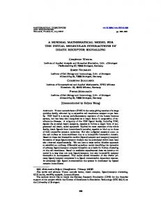
Figure 1 illustrates this idea. Let us take 2 macro–periods with S = S = 2 slots, J = 5 raw materials, J = 6 products, L = 3 tanks and L = 3 lines. Suppose that rmA (raw material A) is used to produce P1 (product 1), rmB produces P2 and P3, rmC produces P4, rmD produces P5 and rmE produces P6. The number of products in lines and raw macro-period 2
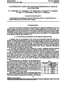
Figure 1: Occupation of tanks and lines slots. materials in tanks cannot be greater than the total number of slots (S = S = 2) in each macro–period. Note that there is not a full slot occupation in figure 1. For instance, only one slot is occupied by raw materials and products, respectively, in tank Tk3 and line L3 during the first macro–period. In the second macro–period, there is no slot occupied in Tk3 and L3. The different slot sizes show us that there are different numbers of products in each slot. In this way, variables and constraints indexed by slots in the model will enable us to describe the lines and tank occupation simultaneously. In a multi–level setting (recall that we have two levels, the tanks and the production lines), it is necessary to coordinate the lots scheduled on one level with the lots scheduled on the other level. For that reason we introduce small micro–periods in a CSLP–like manner, so that a lot on the production line level that must wait for a lot on the tank level requires the tank level lot to be ready at least one micro–period before the start of the production line level lot. Figure2 illustrates this idea starting from the slot occupation in figure 1 and synchronizing the slot scheduled in the two levels. Each macro–period was divided into 5 micro-periods with same length. The acronyms rmA, rmB, rmC, rmD and rmE in figure 2 represent the raw material setup time in a tank. The symbols P1, P2, P3, P4 and P5 represent the processing time of products. For instance, the two slots of Tk1 occupied by rmA indicate that the tank is refilled using the same raw material during the first macro– period. The slot occupation of Tk1 aims to meet the production requirements of P1 in line L1, where the two slots available were occupied by P1. The micro–periods enable us to synchronize the beginning of P1 production in the first slot of L1 with the ending of rmA setup time shown by the first slot of Tk1. Moreover, the micro–period enables us to see when the refilling of Tk1 takes place in the second slot of Tk1. This tank refilling demands the interruption of P1 and the beginning of the second slot occupation of P1, after the end of rmA setup time in Tk1. Taking this into consideration, the model will use constraints and variables indexed by a micro-period that makes it possible to describe this kind of situation. 5
Figure 2: Synchronization between slots in lines and tanks. In short, we can say that the new approach used in the model proposed here is the integration and synchronization of two lot sizing and scheduling problems. This is done using variables and constraints indexed by slots and micro–periods. The slots provide us with the line and tank sequence of occupation. The micro-periods inform us of when this occupation will take place. Slots and micro–periods together enable us to use variables and constraints that integrate and synchronize the lot sizing and scheduling problems in the two levels of this problem. Let us focus on the production lines first to see how this can be expressed formally. As a matter of fact, a particular product can be produced on some lines, but not on all in general. If xjls is a binary variable that indicates for what product j a certain slot s is reserved for, it is easy to express that some reservations will never occur given Lj , the production lines on which product j can be produced: j = 1, . . . , J l ∈ {1, . . . , L}\Lj s = 1, . . . , T · S
xjls = 0
(2)
It is required to have a reservation for each single slot no matter whether or not that slot will indeed be used for producing something: J X
l = 1, . . . , L s = 1, . . . , T · S
xjls = 1
j=1
(3)
If a product j is scheduled for being produced in a certain slot, then there must be a reservation for that particular product. If qjls is the quantity to be produced and pjl is the amount of production time per unit, C, the available time per macro–period, is an upper bound on the time for production, which enable us to link the decision variables qjls and xjls : j = 1, . . . , J l = 1, . . . , L s = 1, . . . , T · S
pjl qjls ≤ Cxjls
6
(4)
Depending on the reservations xjls being made, it is easy to figure out whether or not a setup from product i to product j must take place (zijls indicates this). From this, it is possible to determine the setup time σls to be included just in front of a certain slot: zijls ≥ xjls + xil,s−1 − 1 σls =
J X J X
0 σijl zijls
i=1 j=1
i, j = 1, . . . , J l = 1, . . . , L s = 1, . . . , T · S
(5)
l = 1, . . . , L s = 1, . . . , T · S
(6)
For the first slot of a macro–period t, some setup time ωlt may be at the end of the previous macro–period. If so, the end of the last lot in that previous macro–period must leave sufficient time for this setup time at the end of the previous macro–period: ωlt ≤ σl,(t−1)S+1 m t·T X
t·C −
C m τ xE l,t·S,τ ≥ ωl,t+1
τ =(t−1)T m +1
l = 1, . . . , L t = 1, . . . , T
(7)
l = 1, . . . , L t = 1, . . . , T − 1
(8)
The time capacity per macro–period is constrained to be C time units. Therefore, for each production line, the total sum of production times and setup times in a certain macro–period must not exceed that limit: t·S X
(σls +
J X
pjl qjls ) ≤ C + ωlt
j=1
s=(t−1)S+1
l = 1, . . . , L t = 1, . . . , T
(9)
The inventory balance states that at the end of a macro–period, the number of products on stock equals which we had on stock at the beginning of the period, plus what we have produced, minus the demand. As stated above, we would like to guarantee a feasible solution by allowing shortages. This is modeled by allowing qj0 units being “produced” in the first period without using capacity. Ij1 = Ij0 + qj0 + Ijt = Ij,t−1 +
L X S X
qjls − dj1
l=1 s=1 L t·S X X
qjls − djt
l=1 s=(t−1)S+1
j = 1, . . . , J
(10)
j = 1, . . . , J t = 2, . . . , T
(11)
Two consecutive slots must be scheduled in such a way that precedence constraints among these slots are respected. In other words, the finishing time of one slot, minus the finishing time of the previous slot, must be at least as large as the production time of the lot in the one slot, plus the required setup time in advance of that lot: m t·T X
C m τ xE lsτ
τ =(t−1)T m +1
−
m t·T X
τ =(t−1)T m +1
C
m
τ xE l,s−1,τ
≥ σls +
J X
pjl qjls
j=1
7
l = 1, . . . , L t = 1, . . . , T s = (t − 1)S + 2, . . . , t · S
(12)
m t·T X
C m τ xE l,(t−1)S+1,τ
τ =(t−1)T m +1
≥ (t − 1)C + σl,(t−1)S+1 − ωlt +
J X
pjl qjl,(t−1)S+1
j=1
l = 1, . . . , L t = 1, . . . , T
(13)
To have a well–defined schedule, every slot must have a unique finishing time and a unique starting time for the lot scheduled in that slot: m t·T X
xE lsτ
=1
l = 1, . . . , L t = 1, . . . , T s = (t − 1)S + 1, . . . , t · S
(14)
=1
l = 1, . . . , L t = 1, . . . , T s = (t − 1)S + 1, . . . , t · S
(15)
τ =(t−1)T m +1 m t·T X
xB lsτ
τ =(t−1)T m +1
While xjls indicates whether or not a certain slot is reserved to produce a particular product, uls indicates whether or not that slot is indeed used to schedule a lot. If the slot is not used, then the lot size must be zero. On the other hand, if a real lot is indicated, then at least a small amount ² must be produced: J X
pjl qjls ≤ Culs
j=1
²uls ≤
J X
qjls
j=1
l = 1, . . . , L s = 1, . . . , T · S
(16)
l = 1, . . . , L s = 1, . . . , T · S
(17)
In case a slot is not used, no time should be allocated for that slot, which means that the starting and ending time of the slot are the same, because a lot of size zero is scheduled: m t·T X
τ xE lsτ
−
τ =(t−1)T m +1 m t·T X
m t·T X
τ xB lsτ
≤ T uls
l = 1, . . . , L t = 1, . . . , T s = (t − 1)S + 1, . . . , t · S
(18)
≤ uls
l = 1, . . . , L t = 1, . . . , T s = (t − 1)S + 1, . . . , t · S
(19)
m
τ =(t−1)T m +1
τ xB lsτ
−
m t·T X
τ xE lsτ
τ =(t−1)T m +1
τ =(t−1)T m +1
To avoid some redundancy in the model, whenever a slot is not used, it should start as soon as the previous slot ends: m t·T X
τ xB lsτ −
τ =(t−1)T m +1 m t·T X
l = 1, . . . , L m τ xE ≤ T u ls t = 1, . . . , T l,s−1,τ m τ =(t−1)T +1 s = (t − 1)S + 2, . . . , t · S m t·T X
(20)
m + 1) τ xB l,(t−1)S+1,τ − ((t − 1)T
τ =(t−1)T m +1
l = 1, . . . , L t = 1, . . . , T
≤ T m ul,(t−1)S+1 8
(21)
Another way to avoid redundancy is to enforce that, whenever a slot in used in a macro–period, every other previous slot in the same macro–period must also be used. As a consequence, possibly empty slots in a macro–period are the last ones in that macro– period: l = 1, . . . , L t = 1, . . . , T (22) s = (t − 1)S + 1, . . . , t · S − 1
uls ≥ ul,s+1
The start and the end of a slot must be chosen in such a way that the start indicates the first micro–period in which the lot is produced, if there is a real lot for that slot, and the end indicates the last: m t·T X
²uls +
C m τ xE lsτ
τ =(t−1)T m +1 m t·T X
−
C m τ xB lsτ ≤
pjl qjls
j=1
τ =(t−1)T m +1 m t·T X
J X
l = 1, . . . , L t = 1, . . . , T s = (t − 1)S + 1, . . . , t · S
(23)
l = 1, . . . , L t = 1, . . . , T s = (t − 1)S + 1, . . . , t · S
(24)
C m τ xE lsτ
τ =(t−1)T m +1 m t·T X
−
C
m
τ xB lsτ
≥
J X
pjl qjls − C
m
j=1
τ =(t−1)T m +1
To link the production lines and the tanks, we first figure out which amount of a soft drink being bottled on a line comes from which tank: ¯
qjls =
L X
m t·T X
j = 1, . . . , J l = 1, . . . , L t = 1, . . . , T s = (t − 1)S + 1, . . . , t · S
qkjlsτ
k=1 τ =(t−1)T m +1
(25)
Clearly, the soft drink taken from a tank must be taken during the time window in which the soft drink is filled into bottles: ¯
L X J X
pjl qkjlsτ ≤
m t·T X
C m xE lsτ 0
τ 0 =τ
k=1 j=1
¯
L X J X
l = 1, . . . , L t = 1, . . . , T (26) s = (t − 1)S + 1, . . . , t · S τ = (t − 1)T m + 1, . . . , t · T m
τ X
pjl qkjlsτ ≤
k=1 j=1
l = 1, . . . , L t = 1, . . . , T (27) s = (t − 1)S + 1, . . . , t · S τ = (t − 1)T m + 1, . . . , t · T m
C m xB lsτ 0
τ 0 =(t−1)T m +1
In the first micro–period of a lot, some time δls is reserved for setup or idle time, while the remaining time is production time:
δls =
m t·T X
τ =(t−1)T m +1
τ xE lsτ −
m t·T X
m τ xB lsτ + 1 C
τ =(t−1)T m +1
9
−
J X
l = 1, . . . , L t = 1, . . . , T s = (t − 1)S + 1, . . . , t · S
pjl qjls
j=1 ¯
L X J X
m pjl qkjlsτ ≤ C m − δls + (1 − xB lsτ )C
k=1 j=1
(28)
l = 1, . . . , L t = 1, . . . , T (29) s = (t − 1)S + 1, . . . , t · S τ = (t − 1)T m + 1, . . . , t · T m
Now, we can consider the tanks. Similar to the production lines, not every tank can be used to store every soft drink. What is allowed and what is not, is defined first: j = 1, . . . , J¯ ¯ L ¯j l ∈ {1, . . . , L}\ s = 1, . . . , T · S¯
x¯jks = 0
(30)
At any one given time, only one soft drink can be in a particular tank. We use more or less the same idea as for production lines and consider reservations of slots: ¯
J X
¯ k = 1, . . . , L s = 1, . . . , T · S¯
x¯jks = 1
j=1
(31)
The amount that can be filled into a tank has an upper limit, but for technical reasons, we also have to respect minimum lot sizes whenever something is filled into a tank: j = 1, . . . , J¯ ¯ k = 1, . . . , L s = 1, . . . , T · S¯ j = 1, . . . , J¯ ¯ k = 1, . . . , L s = 1, . . . , T · S¯
q¯jks ≤ Qk x¯jks
q¯jks ≤ Qk u¯ks ¯
J X j=1
¯ k = 1, . . . , L s = 1, . . . , T · S¯
q¯jks ≥ Qk u¯ks
(32)
(33)
(34)
Given the reservations for the slots, it is easy to figure out when sequence-dependent setups occur. In contrast to the production lines, the setup state is not preserved in the tanks, that is, a tank must be setup again (cleaned and filled), even if the same soft drink has been in the tank just before. It must be taken care that, in the model, setups occur only if the tank is really used, because changing the reservation for a tank does not necessarily mean that a setup takes place: i, j = 1, . . . , J¯ ¯ k = 1, . . . , L s = 1, . . . , T · S¯ j = 1, . . . , J¯ ¯ k = 1, . . . , L s = 1, . . . , T · S¯
z¯ijks ≥ x¯jks + x¯ik,s−1 − 2 + u¯ks
x¯jks − x¯jk,s−1 ≤ u¯ks ¯
σ ¯ks =
¯
J X J X
¯ k = 1, . . . , L s = 1, . . . , T · S¯
0 z¯ijks σ ¯ijk
i=1 j=1
10
(35)
(36)
(37)
ω ¯ kt ≤ σ ¯k,(t−1)S+1 ¯
t·S X
σ ¯ks ≤ C + ω ¯ kt
¯ s=(t−1)S+1
t = 1, . . . , T
(38)
¯ k = 1, . . . , L t = 1, . . . , T
(39)
The amount that is filled into a tank must be scheduled, so that the micro–period in which the soft drink comes into the tank is known: j = 1, . . . , J¯ m t·T ¯ X k = 1, . . . , L q¯jks = q¯jksτ (40) t = 1, . . . , T τ =(t−1)T m +1 s = (t − 1)S¯ + 1, . . . , t · S¯ The inventory balance for a tank is simple. What is in the tank at the end of a micro– period is what was in the tank at the beginning of that micro–period, plus what comes into the tank in that micro–period, minus what is taken from that tank for being bottled. Later on we will see that tanks can only be refilled if they are empty. To coordinate the production lines and the tanks, it is required that what is taken out of a tank must have been filled into the tank at least one micro–period ahead: ¯
t·S X
I¯jkτ = I¯jk,τ −1 +
q¯jksτ
¯ s=(t−1)S+1
−
J X L X
t·S X
j = 1, . . . , J¯ ¯ k = 1, . . . , L (41) t = 1, . . . , T τ = (t − 1)T m + 1, . . . , t · T m j = 1, . . . , J¯ ¯ k = 1, . . . , L (42) t = 1, . . . , T τ = (t − 1)T m , . . . , t · T m − 1
rji qkilsτ
i=1 l=1 s=(t−1)S+1
I¯jkτ ≥
J X L X
t·S X
rji qkils,τ +1
i=1 l=1 s=(t−1)S+1
Slots must be scheduled in such a way that the setup time that corresponds to a slot fits into the time window between the end of the previous slot and the end of the slot under consideration. As for the production lines, the setup for the first slot in a macro–period may overlap the macro–period border to the previous macro–period: m t·T X
t·C −
¯ k,t+1 C m τ x¯E ¯ ≥ ω k,t·S,τ
τ =(t−1)T m +1 m t·T X
¯ k = 1, . . . , L t = 1, . . . , T − 1
(43)
¯ k = 1, . . . , L t = 1, . . . , T s = (t − 1)S¯ + 2, . . . , t · S¯
(44)
¯ k = 1, . . . , L t = 1, . . . , T
(45)
C m τ x¯E ksτ
τ =(t−1)T m +1
−
m t·T X
C
m
τ x¯E k,s−1,τ
≥σ ¯ks
τ =(t−1)T m +1 m t·T X
C m τ x¯E ¯ k,(t−1)S+1,τ
τ =(t−1)T m +1
≥ (t − 1)C + σ ¯k,(t−1)S+1 −ω ¯ kt ¯ 11
The end time of a scheduled slot must be unique: m t·T X
x¯E ksτ
¯ k = 1, . . . , L t = 1, . . . , T s = (t − 1)S¯ + 1, . . . , t · S¯
=1
τ =(t−1)T m +1
(46)
The soft drink that is filled into a tank is available for bottling just when the setup of the tank is completed: J X
¯ k = 1, . . . , L t = 1, . . . , T (47) s = (t − 1)S¯ + 1, . . . , t · S¯ τ = (t − 1)T m + 1, . . . , t · T m
q¯jksτ ≤ Qk x¯E ksτ
j=1
The scheduled starting time for a slot must be unique as well: m t·T X
x¯B ksτ = 1
¯ k = 1, . . . , L t = 1, . . . , T s = (t − 1)S¯ + 2, . . . , t · S¯
(48)
x¯B =1 ¯ k,(t−1)S+1,τ
¯ k = 1, . . . , L t = 2, . . . , T
(49)
¯ k = 1, . . . , L
(50)
τ =(t−1)T m +1 m t·T X
τ =(t−2)T m +1 m
T X
x¯B k1τ = 1
τ =1
The time window in which a slot is scheduled must be positive if and only if that slot is used to set up the tank: m t·T X
τ x¯E ksτ
−
τ =(t−1)T m +1
m t·T X
τ x¯B ksτ
τ =(t−1)T m +1
m
≤ T u¯ks m t·T X
¯ k = 1, . . . , L t = 1, . . . , T s = (t − 1)S¯ + 2, . . . , t · S¯
(51)
¯ k = 1, . . . , L t = 2, . . . , T
(52)
¯ k = 1, . . . , L
(53)
¯ k = 1, . . . , L t = 1, . . . , T s = (t − 1)S¯ + 2, . . . , t · S¯
(54)
¯ k = 1, . . . , L t = 2, . . . , T
(55)
τ x¯E ¯ k,(t−1)S+1,τ
τ =(t−1)T m +1 m t·T X
−
τ x¯B ≤ T m u¯k,(t−1)S+1 ¯ ¯ k,(t−1)S+1,τ
τ =(t−2)T m +1 m
m
T X
τ x¯E k1τ
−
T X
m ¯k1 τ x¯B k1τ ≤ T u
τ =1
τ =1 m t·T X
τ x¯B ksτ
τ x¯E ksτ
≤ u¯ks
τ =(t−1)T m +1
τ =(t−1)T m +1 m t·T X
−
m t·T X
τ x¯B ¯ k,(t−1)S+1,τ
τ =(t−2)T m +1
−
m t·T X
≤ u¯k,(t−1)S+1 τ x¯E ¯ ¯ k,(t−1)S+1,τ
τ =(t−1)T m +1
12
m
T X
m
τ x¯B k1τ −
τ =1
T X
¯ k = 1, . . . , L
τ x¯E ¯k1 k1τ ≤ u
(56)
τ =1
Redundancy can be avoided if empty slots are scheduled right after the end of previous slots: m t·T X
τ x¯B ksτ
m t·T X
−
τ x¯E k,s−1,τ
τ =(t−1)T m +1
τ =(t−1)T m +1
≤ T m u¯ks m t·T X
¯ k = 1, . . . , L t = 1, . . . , T s = (t − 1)S + 2, . . . , t · S
(57)
¯ k = 1, . . . , L t = 2, . . . , T
(58)
¯ k = 1, . . . , L
(59)
m τ x¯B + 1) k,(t−1)S+1,τ − ((t − 1)T
τ =(t−2)T m +1
≤ T m u¯k,(t−1)S+1 m
T X
m τ x¯B ¯k1 k1τ − 1 ≤ T u
τ =1
More redundancy can be avoided if we enforce that within a macro–period the unused slots are the last ones: ¯ k = 1, . . . , L t = 1, . . . , T (60) s = (t − 1)S¯ + 1, . . . , t · S¯ − 1
u¯ks ≥ u¯k,s+1
Without loss of generality, we can assume that the time needed to set up a tank is an integer multiple of the time of a micro–period. Hence, the start and end of a slot must be scheduled so that this window equals exactly the time needed to set the tank up: m t·T X
m
C u¯ks +
C m τ x¯E ksτ
τ =(t−1)T m +1 m t·T X
−
C
m
τ x¯B ksτ
=σ ¯ks
τ =(t−1)T m +1 m
C u¯k,(t−1)S+1 + ¯
m t·T X
¯ k = 1, . . . , L t = 1, . . . , T s = (t − 1)S¯ + 2, . . . , t · S¯
(61)
¯ k = 1, . . . , L t = 2, . . . , T
(62)
¯ k = 1, . . . , L
(63)
C m τ x¯E ¯ k,(t−1)S+1,τ
τ =(t−1)T m +1 t·T m
X
−
C m τ x¯B =σ ¯k,(t−1)S+1 ¯ ¯ k,(t−1)S+1,τ
τ =(t−2)T m +1 m
m
C u¯k1 +
T X
C m τ x¯E k1τ
τ =1 m
−
T X
C m τ x¯B ¯k1 − ω ¯ k1 k1τ = σ
τ =1
13
Finally, a tank can only be set up again if it is empty: J¯ X
¯ k = 1, . . . , L t = 1, . . . , T − 1 (64) s = (t − 1)S¯ + 1, . . . , t · S¯ + 1 τ = (t − 1)T m + 1, . . . , t · T m ¯ k = 1, . . . , L s = (T − 1)S¯ + 1, . . . , T · S¯ (65) m m τ = (T − 1)T + 1, . . . , T · T
I¯jk,τ −1 ≤ Qk ((1 − x¯B ¯ks )) ksτ ) + (1 − u
j=1 ¯
J X
¯ks )) I¯jk,τ −1 ≤ Qk ((1 − x¯B ksτ ) + (1 − u
j=1
All decision variables are defined as specified in the appendix.
Computational Results The lack of similar models in the literature led us to create a set of instances for the SITLSP. The parameters adopted are: ¯ = {2, 3}. • L = {2, 3, 4} and L • J = {2, 3, 4} and J¯ = {1, 2}. • S = {2, 3} and S¯ = {2}. • T = {1, 2, 3, 4}, T m = 5 and C m = 1h. • minDem = 500u and maxDem = 10000u, u: product unity. • hj = hj = 1 ($/u). • vjl = v¯jk = 1 ($/u). • Qk = 5000l and Qk = 1000l, l: liter of raw material. A certain combination of parameters L, L, J, J, S and S defines a set of instances. These sets are considered of small-to-moderate sizes if compared to the industrial instances found in soft drink companies. Table 1 presents the values used in each combination. Observe that there are 9 possible combinations for each macro–period T = 1, 2, 3, 4. For L L 2 2 2 2 2 2 3 3 3 3 3 3 4 4 4 4 4 4
J 2 3 4 2 3 4 2 3 4
J 1 2 2 1 2 2 1 2 2
S 2 3 3 2 3 3 2 3 3
S 2 2 2 2 2 2 2 2 2
Table 1: Parameter combination for each set of instances 14
each one of these sets, 10 replications are randomly generated, resulting in 4.9.10 = 360 instances in total. The other parameters of the model are generated from a uniform distribution in the interval [a, b], as shown in Table 2. Parameters 0 σijl σ¯0 ijk pjl rji
Ranges Meaning U [0.5, 1] line setup time U [1, 2] tank setup time U [1000, 2000] process time U [0.3, 3] conversion factor
Table 2: Parameter ranges The computational tests were run on in a Pentium IV microcomputer with 2.8 GHz. Initially, the instances were coded using the modeling language GAMS IDE (version 2.0.10.0) and solved by the solver CPLEX (version 7). The GAMS/CPLEX ran over each instance once during the time limit of 1 hour. Two kinds of problem solutions were returned: the optimal solution or the best feasible solution achieved up to the time limit. Table 3 presents the number of constraints and variables (binaries and continuous) for each set of instances L/L/J/J with T = 1.
Model Continuous Var 263 499 615 452 880 1098 555 1100 1390
Constraints 281 454 512 419 673 764 498 821 924
Table 3: Model statistics for the set of instances with T = 1 The following deviation value was used to compare the solutions: Dev(%) = 100
(Z − Z) Z
(66)
where Z is the final solution value returned by GAMS/CPLEX and Z is the lower bound value also determined by GAMS/CPLEX. Table 4 shows the GAMS/CPLEX results for the set of instances with T = 1. Each combination L/L/J/J represents a set containing 10 instances. The second column shows the number of optimal solutions found among the 10 instances evaluated. The average (Avg), maximum (Max), minimum(Min) values and the standard deviation (Std) of Dev and CPU are also listed in the table. Note in the table that the runtime limit of 3600 seconds was reached for certain instances (see column Max), however, GAMS/CPLEX was able to solve most of the problem instances optimally with T = 1 (77 out of 90 instances) within this time limit. 15
Table 5: Model statistics for the set of instances with T = 2 Table 5 shows the model statistics for the set of instances with T = 2. Table 6 presents the corresponding GAMS/CPLEX results obtained for T = 2. The GAMS/CPLEX starts L/L/J/J 2/2/2/1 2/2/3/2 2/2/4/2 3/2/2/1 3/2/3/2 3/2/4/2 4/2/2/1 4/2/3/2 4/2/4/2
Table 6: GAMS/CPLEX results for the set of instances with T = 2 having difficulties in finding an optimal solution within the time limit for this set - note that only 25 out of 90 instances were optimally solved. Moreover, the required average CPU runtimes largely increase. Most of the solutions obtained consist of the best feasible 16
solutions found by the branch & cut algorithm up to the time limit. This is expected in some sense because of the increase in the number of constraints and variables of the model for each instance (table 5). This behavior becomes worse for the set of instances with T = 3, 4, whose results are presented in tables 7 and 8. The GAMS/CPLEX was unable to find optimal solutions
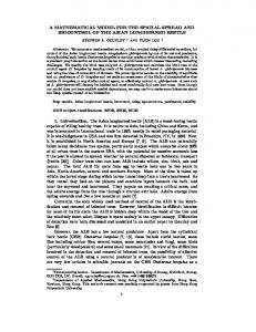
Table 8: GAMS/CPLEX results for the set of instances with T = 4 in most of these problem instances within 1 hour. The increase in the deviation values show us that the quality of the best feasible solution obtained becomes worse than in the previous sets of instances. Tables 9 and 10 show the model statistics for the sets of instances with T = 3, 4. The complexity of the model proposed here, associated with the high number of variables and constraints in the sets of instances with T = 3, 4, explains the hardness found by the branch & cut algorithm to determine optimal solutions during the time limit of 1 hour. Figure 3 uses the set of instances 4/2/4/2 as an example to illustrate the number of variables and constraints when T = 1, 2, 3, 4. Observe that the number of binary variables reaches something near 1000 in the last macro–period. The number of continuous variables starts around 1000 when T = 1 and it is greater than 5000 when T = 4. The number of constraints is near 1000 for T = 1 and almost 4000 for T = 4. 17
Table 10: Model statistics for the set of instances with T = 4 6000
Total Number
5000
Binaries Var.
4000 3000
Contínuous Var.
2000
Constrains 1000 0 1
2
3 Macro-periods
4
Figure 3: Variables and constraints in the set of instances 4/2/4/2.
Conclusion In this paper we present a mathematical model able to describe an industrial problem found in some industrial settings, such as in soft drink companies. It is a two level production problem where, in each level, a lot sizing and scheduling problem with parallel machines, capacity constraints and sequence-dependent setup costs and times has to be solved. The solutions in each level are integrated because the decisions made in one level have consequences for the other. These solutions are also synchronized because 18
the scheduling in both levels have to be compatible throughout the time periods of the planning horizon. This problem was called a Synchronized and Integrated Two-Levels Lot Sizing and Scheduling Problem (SITLSP) here. The first contribution of this work was to propose a new model to represent the synchronization and integration features in our problem. The constraints established are not new, but they are assembled the first time to describe lots and micro-periods simultaneously in a two levels integrated approach. The model was evaluated here using instances considered of small-to-moderate sizes if compared to the industrial instances of soft drink companies. Our goal was to find solutions within 1 hour of computer runtime in each instance. The software GAMS/CPLEX was used to obtain optimal solutions or the best feasible solution at least. This exact solution approach was able to return the optimal solution only in small size instances (T = 1, 2). In most part of the instances, the best feasible solution found was returned at the end of the time limit. It is worth mentioning that the CPLEX version used in the experiments (CPLEX 7.0) is out-of-date and the newest version (CPLEX 10.0) could result in better performances The mixed-integer linear formulation proposed is large and complex because of its vast set of parameters, variables and constraints. This became hard for the exact solution approach to find optimal solutions when the parameters of the model increases. An interesting perspective for future research is to develop effective heuristic methods to deal with this problem. Following this line of research, the difficulties found in determining exact solutions led us to develop a genetic algorithm to deal with such a problem. The results obtained using this approach are being compiled and they will be reported in a forthcoming paper.
Acknowledgement We are indebted to Fl´avio A. M. Veronese from Companhia de Bebidas Ipiranga, Ribeir˜ao Preto, Brazil, for his kind collaboration. This research was partially supported by FAPESP (grant no. 00/02609–2) and CNPq (grant no. 303956/2003-8).
A
Symbols for Parameters and Decision Variables
A.1
General Parameters
T Number of macro–periods C Capacity (in time units) within a macro–period T m Number of micro–periods per macro–period C m Capacity (in time units) within a micro–period (C = T m C m ) ² A very small positive, real–valued number M A very large number
19
A.2
Parameters for the Production Lines
J Number of products L Number of parallel lines Lj Set of lines on which product j can be produced S Upper bound on the number of lots per macro–period, i.e. the number of slots djt Demand for product j at the end of macro–period t sijl Sequence-dependent setup cost coefficient for a setup from product i to j on line l (sjjl = 0) hj Holding cost coefficient for having one unit of product j in inventory at the end of a macro–period vjl Production cost coefficient for producing one unit of product j on line l pjl Production time needed to produce one unit of product j in line l (assumption: pjl ≤ C m ) xjl0 = 1, if line l is set up for product j at the beginning of the planning horizon 0 0 0 σijl Setup time for setting line l up from product i to product j (σijl ≤ C; σjjl = 0)
ωl1 Setup time for the first slot on line l in macro–period 1 that has already been performed before macro–period 1 starts (note: if ωl1 > 0 then values xjl1 are already known and these variables should be set accordingly) Ij0 Initial inventory of product j
A.3
Decision Variables for the Production Lines
zijls = 1, if line l is set up from product i to j at the beginning of slot s; 0, otherwise (zijls ≥ 0 is sufficient) Ijt Amount of product j in inventory at the end of macro–period t qjls Number of products j being produced on line l in slot s xjls = 1, if slot s on line l can be used to produce product j; 0, otherwise uls = 1, if a positive production amount is produced in slot s in production line l (0, otherwise) σls Setup time at line l at the beginning of slot s ωlt Setup time for the first slot on production line l in macro–period t that is scheduled at the end of macro–period t − 1 xE lsτ = 1, if lot s (which belongs to a single macro–period t) on line l ends in micro–period τ 20
xB lsτ = 1, if lot s (which belongs to a single macro–period t) on line l begins in micro– period τ δls Time in the first micro–period of a lot which is reserved for setup time and idle time qj0 Shortage of product j
A.4
Parameters for the Tanks
J¯ Number of raw materials ¯ Number of parallel tanks L ¯ j Set of tanks in which raw material j can be stored L S¯ Upper bound on the number of lots per macro–period, i.e. the number of slots s¯ijk Sequence-dependent setup cost coefficient for a setup from raw material i to j in tank l ¯ j Holding cost coefficient for having one unit of raw material j in inventory at the h end of a macro–period v¯jk Production cost coefficient for filling one unit of raw material j in tank k x¯jk0 = 1, if tank k is set up for raw material j at the beginning of the planning horizon 0 0 σ ¯ijk Setup time for setting tank k up from raw material i to raw material j (¯ σijk ≤ C) 0 m (w.l.o.g. σ ¯ijk is an integer multiple of C )
ω ¯ k1 Setup time for the first slot on tank k in macro–period 1 that has already been performed before macro–period 1 starts (note: if ω ¯ k1 > 0 then values x¯jk1 are already known and these variables should be set accordingly) I¯jk0 Initial inventory of raw material j in tank k Qk Maximum amount to be filled in tank k Qk Minimum amount to be filled in tank k
A.5
Decision Variables for the Tanks
z¯ijks = 1, if tank k is set up from raw material i to j at the beginning of slot s; 0, otherwise (¯ zijks ≥ 0 is sufficient) I¯jkτ Amount of raw material j in tank k at the end of micro–period τ q¯jks Amount of raw material j being filled in tank k in slot s q¯jksτ Amount of raw material j being filled in tank k in slot s in micro–period τ x¯jks = 1, if slot s can be used to fill raw material j in tank k; 0, otherwise
21
u¯ks = 1, if slot s is used to fill raw material in tank k; 0, otherwise σ ¯ks Setup time, i.e. the time for cleaning and filling the tank up, at tank k at the beginning of slot s ω ¯ kt Setup time, i.e. the time for cleaning and filling the tank up, for the first slot on tank k in macro–period t that is scheduled at the end of macro–period t − 1 x¯E ksτ = 1, if lot s — a setup, i.e. cleaning und filling the tank up — (which belongs to a single macro–period t) at tank k ends in micro–period τ x¯B ksτ = 1, if lot s — a setup, i.e. cleaning und filling the tank up — (which belongs to a single macro–period t) at tank k begins in micro–period τ
A.6
Parameters for Linking Production Lines and Tanks
rji Amount of raw material j to produce one unit of product i
A.7
Decision Variables for Linking Production Lines and Tanks
qkjlsτ Amount of product j, which is produced on line l in micro–period τ and which belongs to lot s, that uses raw material from tank k
References [1] Berreta, R. E., Frana, P.M., Armentano, V.A., (2005), Metaheuristic approaches for the multilevel resource-constrained lot-sizing problem with setup and lead times, Asia-Pacific Journal of Operational Research, Vol. 22(2), pp. 261–286. [2] Campbell, G.M., (1992), Using Short–Term Dedication for Scheduling Multiple Products on Parallel Machines, Production and Operations Management, Vol. 1, pp. 295–307. [3] Carreno, J. J. , (1990), Economic Lot Scheduling for Multiple Products on Parallel Identical Processors, Management Science, Vol. 36, pp. 348–358. [4] de Matta, R., Guignard, M., (1995), The Performance of Rolling Production Schedules in a Process Industry, IIE Transactions, Vol. 27, pp. 564–573. [5] Drexl, A., Kimms, A., (1997), Lot Sizing and Scheduling — Survey and Extensions, European Journal of Operational Research, Vol. 99, pp. 221–235. [6] Fleischmann, B., (1994), The Discrete Lot–Sizing and Scheduling Problem with Sequence–Dependent Setup Costs, European Journal of Operational Research, Vol. 75, pp. 395–404. [7] Haase, K., Kimms, A., (2000), Lot Sizing and Scheduling with Sequence- Dependent Setup Costs and Times and Efficient Rescheduling Opportunities, International Journal of Production Economics, Vol. 66, pp. 159–169.
22
[8] Kang, S., Malik, K. and Thomas, L. J., (1999), Lotsizing and Scheduling on Parallel Machines with Sequence–Dependent Setup Costs, Management Science, Vol. 45, pp. 273–289. [9] Kimms, A., (1997), Demand Shuffle — A Method for Multi–Level Proportional Lot Sizing and Scheduling, Naval Research Logistics, Vol. 44, pp. 319–340. [10] Kimms, A., (1997), Multi–Level Lot Sizing and Scheduling, Heidelberg, Physica. [11] Kuhn, H., Quadt, D., (2002), Lot Sizing and Scheduling in Semiconductor Assembly — A Hierarchical Planning Approach, in: Mackulak, G. T., Fowler, J. W. , Sch¨omig, A., (eds.), Proceedings of the International Conference on Modeling and Analysis of Semiconductor Manufacturing, Tempe, USA, pp. 211–216. [12] Meyr, H., (1999), Simultane Losgr¨ossen– und Reihenfolgeplanung f¨ ur kontinuierliche Produktionslinien, Deutscher Universit¨ats–Verlag. [13] Meyr, H., (2002), Simultaneous Lotsizing and Scheduling on Parallel Machines, European Journal of Operational Research, Vol. 139, pp. 277–292. [14] Meyr, H., (2003), Simultane Losgr¨ossen– und Reihenfolgeplanung bei mehrstufiger kontinuierlicher Fertigung, Working Paper, University of Augsburg. [15] Quadt, D., Kuhn, H., (2003), Production Planning in Semiconductor Assembly, Working Paper, Catholic University of Eichst¨att–Ingolstadt. [16] Stadtler, H., (1996), Mixed Integer Programming Model Formulations for Dynamic Multi-Item Multi–Level Capacitated Lotsizing, European Journal of Operational Research, Vol. 94, pp. 561-581. [17] Tempelmeier, H., Derstroff, (1996), A Lagrangean–Based Heuristic for Dynamic Multilevel Multiitem Constrained Lotsizing with Setup Times, Management Science, Vol. 42, pp. 738–757. [18] Wolsey, L. A. , (2002), Solving Multi–Item Lot–Sizing Problems with an MIP Solver Using Classification and Reformulation, Management Science, Vol. 48, pp. 1587– 1602.