A Mathematical Model with a Modified Logistic ...

Theoretical Population Biology 56, 301306 (1999) Article ID tpbi.1999.1426, available online at http:www.idealibrary.com on

A Mathematical Model with a Modified Logistic Approach for Singly Peaked Population Processes Ryoitiro Huzimura 1 Department of Economics, Osaka Gakuin University, 2-36-1 Kishibe-minami, Suita-shi, Osaka 564-8511, Japan

and Toyoki Matsuyama 2 Department of Physics, Nara University of Education, Takabatake-cho, Nara 630-8528, Japan Received August 17, 1998

When a small number of individuals of a single species are confined in a closed space with a limited amount of indispensable resources, breeding may start initially under suitable conditions, and after peaking, the population should go extinct as the resources are exhausted. Starting with the logistic equation and assuming that the carrying capacity of the environment is a function of the amount of resources, a mathematical model describing such a pattern of population change is obtained. An application of this model to a typical set of population records, that of deer herds by V. B. Scheffer (1951, Sci. Monthly 73, 356362) and E. C. O'Roke and F. N. Hamerstrom (1948, J. Wildlife Management 12, 7886), yields estimates of the initial amount of indispensable food and its availability or nutritional efficiency which were previously unspecified. ] 1999 Academic Press

time and the populations first increased nearly exponentially to reach a peak and then decreased or finally went extinct. The change was considered to be fluctuation or overabundance from the sigmoidal pattern and ascribed to changes in the reproduction rate andor mortality due to unspecified reasons. But, such patterns should be generally observable if living organisms are confined in a closed space with a constant amount of growth resources which are actually not reproducible although initially given. Effects of food availability or resource limitation on population dynamics are one of recent concerns (e.g., Ogushi and Sawada, 1985; Edgar and Aoki, 1993). To our knowledge, however, rather few mathematical models have been studied to analyse such patterns of population change and the carrying capacity for

INTRODUCTION The logistic or the LotkaVolterra model has long been a mathematical frame work for studying population dynamics tending to a stationary or oscillating equilibrium due to intra- or interspecific interactions (e.g., Pielou, 1974; Begon et al., 1996; Borrelli and Coleman, 1996; Glesson and Wilson, 1986; Reed et al., 1996). Also, there is another pattern of population change which is singly peaked. A typical one is the population change of deer herds observed by Scheffer (1951). It was reported that the deer were freed in closed spaces at some definite 1 2

Fax: 0081-06-6382-4363. Fax: 0081-0742-27-9289. E-mail: matsuyatnara-edu.ac.jp.

301

0040-580999 K30.00 Copyright ] 1999 by Academic Press All rights of reproduction in any form reserved.

302

Huzimura and Matsuyama

population has been traditionally assumed to be a constant characterizing its environment. In this report, we propose a new mathematical model to interpret such a pattern of population change by introducing the new assumption that the carrying capacity is a function of the amount of resources. After its formulation and its application to the deer herd population, we discuss several characteristics of our model as compared with the existing models.

MATHEMATICAL MODELS We start with the logistic equation for a single species living in some limited space, N 1 dN , =r 1& N dt K

\

+

(1)

where N is the population size of the species, r the potential net reproduction rate, and K the carrying capacity of the population. Now we assume that the carrying capacity depends on the amount of indispensable resources in the space for the organisms and the resources are consumed by the organisms after they begin to live. In such a situation, we may assume that the carrying capacity is a function of the amount (X ) of the resource, K= f (X ). Thus, we have N 1 dN =r 1& . N dt f (X )

\

+

(2)

We may further assume that the decreasing rate of X is proportional to the population size and the reproduction rate of the resources is negligible compared with the consumption rate, i.e., dX =&aN, dt

(3)

where a (>0) is the consumption rate of the resources per individual per unit time. From Eqs. (2) and (3), we have r N =r(t&t 0 )+ ln N0 a

|

X X0

dX , f (X )

(4)

where N 0 , X 0 , and t 0 are the initial values of N, X, and t, respectively. There may be various choices for f (X ) as an integrable function which represents a possible

dependence of carrying capacity on resources. We choose here the simplest, a linear function f (X )=bX, with the proportional constant b ( >0), which we call the nutritional efficiency. Thus we have N(t)=N 0

X(t) X0

_ &

rab

exp(rt),

(5)

with t 0 =0. Equation (5) predicts that the amount of resources per individual, XN, in the case of a=rb, decreases exponentially with time from the initial value X 0 N 0 . Solving the simultaneous Eqs. (3) and (5), we obtain the following solutions: For a=rb,

_

N(t)=N 0 exp rt+

a N0 [1&exp(rt)] , r X0

&

(6)

and for a{rb, a 1 N0 [1&exp(rt)] & r b X0

_ \ +

N(t)=N 0 1+

&

r(ab&r)

_exp(rt).

(7)

The N(t) curve given by Eq. (6) or Eq. (7) has a single peak for a limited range or combinations of parameters a, b, r, X 0 , and N 0 . The range giving the single peak is determined from the extreme condition of N(t). The solution (6) for a=rb has a peak if rX 0 aN 0 >1. We note that rX 0 aN 0 =bX 0 N 0 in this case. The maximum of N is given by Nm =

rX 0 aN 0 &1 , exp a rX 0

\

+

(8)

at time t m =(1r) ln(rX 0 aN 0 ). For a{rb, the peak exists again when bX 0 N 0 >1. The maximum is N0 1 r+(ab&r) ab bX 0

_ { rX r _ \aN +1&ab+

N m =N 0

0

=&

r(ab&r)

(9)

0

with t m =(1r) ln(rX 0 aN 0 +1&rab). We show the range where a single peak exists on the (N 0 X 0 , b) plane in Fig. 1. It should be noted that our model is soluble exactly. We also note that it is scale invariant under the change of (a, 1b, X 0 ) into (*a, *b, *X 0 ) with an arbitrary constant *, and the units of X define the units of a and b.

Singly Peaked Population Processes

303

FIG. 1. The range in which the condition giving a peak in N(t) curves is fulfilled: b>N 0 X 0 . Notation is defined in the text.

APPLICATION TO THE DEER POPULATIONS What can be analysed by the present model? To show this, we apply the model to the population changes of reindeer on St. Paul Island (SPI) from 1911 to 1950 and on St. George Island (SGI) from 1911 to 1949 (Scheffer, 1951). The population data are well known to be from an ideal observation in an outdoor laboratory where the animals lived under small hunting pressure and were free of predator attack for 40 years; a definite number of animal were placed in the closed spaces at a definite time, after which the population showed singly peaked changes. The accuracy of the numbers was estimated to be about 10 0. We also apply the model to the population change of white-tailed deer at the George Reserve of the University of Michigan (GRM) which showed a similar trend from 1928 to 1947 (O'Roke and Hamerstrom, 1948). For the application, we need to fix one of three parameters, a, b, and X 0 , and we need to assume the presence of an indispensable resource for the animals. We may assume that it was lichen at least for the SPI herd. This is because lichen was considered to be the key forage for reindeer, especially in winter (Scheffer, 1951). The grass disappeared on SPI 40 years after the introduction of reindeer, which was regarded as the cause of the extinction of the reindeer. We may apply Eq. (3) here without adding any reproduction term for plant breeding since it was reported that recovery of the lichen range may take 15 or 20 years. A caribou is reported to eat 4.5 kg of lichen a day (Bandfield, 1996). We infer that real values of the consumption rate of the three deer herds are near to this value since they belong to the same family (a

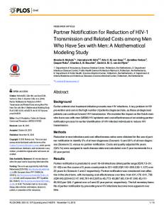
FIG. 2. Population curves obtained with Eqs. (6) and (7) in the text to fit the population records of the three deer herds. The nutritional efficiency (b), the initial stock of indispensable food (X 0 ), and the potential reproduction rate (r) which are defined in the text are optimized. (A) Reindeer on St. Paul Island (Scheffer, 1951); (B) reindeer on St. George Island (Scheffer, 1951); and (C) white-tailed deer in the George Reserve, Michigan (O'Roke and Hamerstrom, 1948).

304

Huzimura and Matsuyama

TABLE I Population Data of Three Deer Herds

Herd St. Paul Island reindeer St. George Island reindeer George Reserve w.t. deer

Habitat area (acres)

N0

Nm

r( y &1 )

b (individualton)

X 0 (tons)

K0

26,500 22,400 1,200

25 15 6

2046 222 211

0.182 0.469 0.740

0.111 0.0512 0.0561

37,000 4,460 4,150

4090 229 233

Note. The habitat area and the initial and maximum population sizes (N 0 and N m ) are from Scheffer (1951) and O'Roke and Hamerstrom (1948). The nutritional efficiency (b), the initial stock of indispensable food (X 0 ), and the reproduction rate (r) which are defined in text are obtained in this work after direct search optimization of the theoretical curve (Eqs. (6) and (7) in the text) to fit the population records in the references and shown with significant figures of three digits. The consumption rate of indispensable food (a) is fixed to be 1.64 tons per year per individual for the three herds. K 0 ( =bX 0 ) is the initial carrying capacity given in the text.

Japanese deer is reported to eat 11 kg of grass a day). As the choice of this value is not essential when considering the actual population, we use a=1.64 tons a year per individual for the three herds. The population change (N) of the SPI reindeer from Scheffer's table is shown in Fig. 2A with empty circles. To fit the curve of Eq. (7), we use direct search of optimization (DSO) for three parameters, r, b, and X 0 , and we obtain r=0.182 per year, b=0.111 individual per ton, and X 0 =37,000 tons. We notice here some deviation of the curve from the data points which might be caused by changes in hunting effects or weather. We cannot clarify the reason at present, however. After a similar application of DSO to the population on SGI and that in GRM, the optimized curves are compared with the observed data in Figs. 2B and 2C. All parameters thus obtained are summarized in Table I together with the areas of three habitats and the respective initial and maximum population sizes. Now we explain some characteristics of the population processes, referring to the figures and to Table I. The most significant result in Table I is that the initial stock X 0 on SPI is more than eight times larger than that on SGI although the land areas are almost the same. In the present model, the deviation of X 0 is proportional to that of a due to the scale invariance of the parameters mentioned above. However, this difference in the X 0 's is much more than can be caused by a probable difference in the a's. Rather, this may correspond to an approximately 10 times larger N m observed on SPI than on SGI and suggests that SPI was much more fertile than SGI. Scheffer remarked on some environmental differences between the two islands. Here we propose that the initial values of the carrying capacity are given by K 0 =bX 0 (data also included in Table I). K 0 is free from the effect of ambiguity of a. The significant difference between the

K 0 's of SPI and SGI in Table I also supports the above view. We find next that the net reproduction rate r of the SPI herd is much smaller than that of SGI which further is smaller than that of GRM. Values of r are free from the effects of a. A biological reason may exist for the differences in r, although we cannot explain it now. The b value of the SPI herd is about twice that of the SGI herd (and the GRM herd). However, this difference might be caused by any difference in possible a values. Further, we find significant differences between population processes on SPI and on SGI (and in GRM): The population on SPI increased rather slowly and went extinct steeply after the maximum while that on SGI increased fast and decayed slowly. For the SPI herd, the ratio of the obtained r to the b value is very near to the a value, meaning that the curve fitting for SPI reindeer is attained with Eq. (6) or as the case a=rb, as far as the a value is acceptable. In contrast with this, some similarities are found in the population processes of SGI

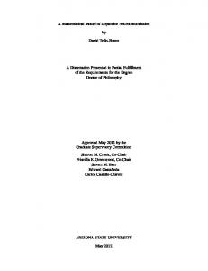
FIG. 3. The maximum size of deer populations observed (N m ) vs the initial amount of indispensable food (X 0 ) estimated in the text.

305

Singly Peaked Population Processes TABLE II The Estimations of N m X 0 of Three Deer Herds Herd St. Paul Island reindeer St. George Island reindeer George Reserve w.t. deer

N m(DATA)X 0

N m(LNR)X 0

N m(DSO)X 0

0.0553 0.0498 0.0508

0.0407 0.0352 0.0417

0.0409 0.0356 0.0419

Note. N m(DATA), N m(LNR), and N m(DSO) are defined in the text. They are divided by X 0 , which takes the value corresponding to each herd in Table I.

reindeer and GRM white-tailed deer: rb is much less than the assumed a for both herds, meaning that the fitting is realized with Eq. (7) or as the case a