SS symmetry Article
A Logistic Based Mathematical Model to Optimize Duplicate Elimination Ratio in Content Defined Chunking Based Big Data Storage System Longxiang Wang 1 , Xiaoshe Dong 1 , Xingjun Zhang 1, *, Fuliang Guo 1 , Yinfeng Wang 2 and Weifeng Gong 3 1
2 3
*
The School of Electronic and Information Engineering, Xi’an Jiaotong University, Xi’an 710049, China;
[email protected] (L.W.);
[email protected] (X.D.);
[email protected] (F.G.) The Shenzhen Institute of Information Technology, Shenzhen, 518172, China;
[email protected] State Key Laboratory of High-End Server & Storage Technology, Jinan 250101, China;
[email protected] Correspondence:
[email protected]; Tel.: +86-029-8266-8478
Academic Editors: Doo-Soon Park and Shu-Ching Chen Received: 31 May 2016; Accepted: 15 July 2016; Published: 21 July 2016
Abstract: Deduplication is an efficient data reduction technique, and it is used to mitigate the problem of huge data volume in big data storage systems. Content defined chunking (CDC) is the most widely used algorithm in deduplication systems. The expected chunk size is an important parameter of CDC, and it influences the duplicate elimination ratio (DER) significantly. We collected two realistic datasets to perform an experiment. The experimental results showed that the current approach of setting the expected chunk size to 4 KB or 8 KB empirically cannot optimize DER. Therefore, we present a logistic based mathematical model to reveal the hidden relationship between the expected chunk size and the DER. This model provides a theoretical basis for optimizing DER by setting the expected chunk size reasonably. We used the collected datasets to verify this model. The experimental results showed that the R2 values, which describe the goodness of fit, are above 0.9, validating the correctness of this mathematic model. Based on the DER model, we discussed how to make DER close to the optimum by setting the expected chunk size reasonably. Keywords: storage system; deduplication; duplication elimination ratio; content defined chunking
1. Introduction Deduplication is an efficient data reduction technique, and it is used to mitigate the problem of huge data volume in big data storage systems. At present, deduplication is widely used in secondary storage systems such as backup or archival systems [1–4], and is also gradually used in primary storage systems, such as file systems [5,6]. Content defined chunking (CDC) [7] can achieve high duplicate elimination ratios (DERs), and therefore is the most widely used data chunking algorithm. DER indicates the ratio of the eliminated data processed by the deduplication, and is used as an essential indicator to evaluate the deduplication effect. Therefore, improving DER has been an important research area for the storage community. After a deduplication process, a storage system needs to store unique and meta data. The unique data refers to the data that is judged as new by a deduplication process. The metadata refers to the data that saves the address information of a data chunk that is used to rebuild a data stream. This will occur while a restoration is needed in a backup system, or a file read is requested in a primary storage system. The expected chunk size is an important parameter in CDC algorithms and needs to be set before the deduplication is enabled. A smaller chunk size results in a large number of metadata and hence requires a significant amount of storage space, but it will reduce the unique data size, and vice versa. Thus, the expected chunk Symmetry 2016, 8, 69; doi:10.3390/sym8070069
www.mdpi.com/journal/symmetry
Symmetry 2016, 8, 69
2 of 12
size will influence DER significantly and is an important parameter in CDC [8]. The researcher has pointed out that a reasonable setting of the expected chunk size could increase DER significantly [9]. To increase DER, the researcher has been focusing on improving chunking algorithms; however, few studies have been done on how to set the expected chunk size reasonably to increase DER. Nowadays, researchers consider 4 KB or 8 KB empirically as the reasonable expected chunk size. However, these values lack both theoretical proof and verification with realistic datasets. To verify whether setting the expected chunk size to 4 KB or 8 KB can improve DER, we collected two realistic datasets to perform the experiment. The datasets are: (1) Linux kernel source codes; and (2) multiple SQLite backup data while running the Transaction Processing Performance Council-C (TPC-C) benchmark. The experimental results showed that setting the expected chunk size to 4 KB or 8 KB cannot optimize DER. To study how to set the expected chunk size reasonably in order to optimize DER, we propose a logistic based mathematical model to reveal the hidden relationship between the expected chunk size and the DER. Two realistic datasets were used to verify this model. The experimental results showed that the R2 values, which describe the goodness of fit, are above 0.9, validating the correctness of this mathematic model. Based on this model, we discussed how to set the expected chunk size to make DER close to the optimum. Our contributions in this paper are the following: (1) (2)
(3)
With two realistic datasets, we showed that the expected chunk size 4 KB or 8 KB that is currently considered reasonable, cannot optimize DER. We present a logistic based mathematical model to reveal the hidden relationship between the DER and the expected chunk size. The experimental results with two realistic datasets showed that this mathematical model is correct. Based on the proposed model, we discussed how to set the expected chunk size to make DER close to the optimum.
2. Related Work DER is an essential metric to evaluate the deduplication effect. Thus, to increase DER is an important study in the deduplication research area. At present, researchers mainly focus on improving data chunking algorithms to increase DER. The purpose of data chunking algorithms is to divide a data stream into a series of chunks that are used as the basic units to detect duplicated data. Currently, there are three kinds of data chunking algorithms: (1) single instance store (SIS)— under this method, the whole file is used as the basic unit to perform a deduplication. The representatives are SIS in Windows 2000 (NT 5.0, Microsoft, Redmond, WA, USA) [10] and DeDu [11]. The problem of the single instance store is its low DER; (2) fixed sized partitioning (FSP)—this algorithm divides the file into fixed sized chunks, which are used as basic units to perform a deduplication. The representatives of FSP are Venti [4] and Oceanstore [12]. Compared with SIS, FSP improved DER significantly. However, the effectiveness of this approach on DER is highly sensitive to the sequence of edits and modifications performed on consecutive versions of an object. For example, an insertion of a single byte at the beginning of a file can change the content of all chunks in the file resulting in no sharing with existing chunking; and (3) content defined chunking (CDC). CDC employs Rabin’s fingerprints [13] to choose partition points in the object. Using fingerprints allows CDC to “remember” the relative points at which the object was partitioned in previous versions without maintaining any state information. By picking the same relative points in the object to be chunk boundaries, CDC localizes the new chunks created in every version to regions where changes have been made, keeping all other chunks the same. CDC was first applied in LBFS (A Low-bandwidth Network File System) [7]. Moreover, lots of chunking algorithms are developed based on CDC to improve DER [9,14–16]. Because CDC can avoid the problem of data shifting and is widely used, and is also the basic foundation of many improved algorithms, we study the influence of expected chunk size on DER in CDC based deduplication. The expected chunk size is an important parameter in CDC algorithms, and will affect DER significantly. Thus, it is important to study how to set the expected chunk size reasonably to
Symmetry 2016, 8, 69
3 of 12
improve DER. Nowadays, researchers suggest setting the expected chunk size by rule of thumb. For example, 4 KB [17] or 8 KB [3,7,18] are considered reasonable by some researchers; Symantec Storage Foundation 7.0 (Mountain View, CA, USA) recommends a chunk size of 16 KB or higher [19]; IBM (Armonk, NY, USA) mentioned the average chunk size for most deduplicated files is about 100 KB [20]. However, these expected chunk sizes lack either theoretical proof or experimental evaluation. Suzaki [21] studied the effect of chunk size from 4 KB to 512 KB on Input/Output (I/O) optimization by experiments, and showed large chunks (256 KB) were effective. However, the main concern of Suzaki’s work is to optimize I/O rather than DER by setting chunk size, whereas, we focus on the impact of chunk size on DER in this paper. 3. Background 3.1. The Symbol Definitions In Table 1, we defined the symbols that will be used in this paper. Table 1. The symbol definitions. The Name of Symbol
The Meaning of Symbol
x µ So W Nm Sm Su Sd m L k x0
The mask length in binary The expected chunk size The original data size The size of the sliding window The metadata number after deduplication The metadata size after deduplication The unique and fingerprint index data size after deduplication The total data size after deduplication The single metadata size The upper bound of the logistic function;; The steepness of the logistic curve The x-value of the logistic curve’s midpoint
3.2. The Principal of CDC In this paper, our study was based on the original implementation of CDC, which was first proposed in LBFS [7]. The principal of the CDC algorithm is shown in Figure 1. A 48 byte window slides continuously from the beginning of the data stream. The rabin fingerprint [13] of the current window data is calculated and then this fingeprint is judged on whether its low-order x bits equals a magic value. Thus, the boundary can be judged by whether the condition rabin_fp & mask==mask-1 is met. The rabin_fp represents the rabin fingerprint of the current window data; mask is a predefined binary value and is used to obtain the low-order x bits of the fingerprint. For example, if mask is set to 1111 in binary, the low-order 4 bits will be obtained. The magic value could be set to mask-1 or any value less than or equal to mask. If the condition is met, the last byte of the current window is used as the boundary of the chunk. After the window sliding finished, the formed boundaries divide the data stream into a series of data chunks with variable lengths. To avoid the chunks being too large or too small, the maximum and minimum value of the chunks need to be set. The window slides from a minimum chunk size position, and if the chunk size is bigger than maximum, the last byte of the current window is set as the boundary enforced.
Symmetry 2016, 8, 69 Symmetry 2016, 8, 69
4 of 12 4 of 12
Calculate the rabin fingerprint of current 48 bytes window data and judge whether the boundary is found
...
Data stream
One byte
Move the sliding window by one byte
...
Data stream
... ...
...
Data stream
The found boundaries (Rabin fingerprint of the sliding window data & mask==mask-1) Chunking results
...
Chunk 1
...
Chunk 2
Data stream
Chunk 3
Figure 1. The principal of Content defined chunking (CDC) algorithm. Figure 1. The principal of Content defined chunking (CDC) algorithm.
3.3. The The Expected Expected Chunk Chunk Size Size 3.3. The process algorithm is to a window by one the current The processofofthe theCDC CDC algorithm is slide to slide a window bybyte oneand bytejudge and whether judge whether the position is a boundary. Since the rabin hash function [13] generates a fingerprint with input data current position is a boundary. Since the rabin hash function [13] generates a fingerprint with input uniformly, the probability that low-order x bitsxofbits a region’s fingerprint equals a chosen valuevalue is 1/2isx . data uniformly, the probability that low-order of a region’s fingerprint equals a chosen This chunking process can be a Bernoulli trial; thus, thethe expected boundaries number X 1/2x. This chunking process canconsidered be considered a Bernoulli trial; thus, expected boundaries number obeys Binomial distribution, as X obeys Binomial distribution, as X „ bpS ´ W ` 1, 1{2x q (1) X ~ b(S W 1,1/ 2x ) (1) In Equation (1), S is the length of the data stream; W is the size of the sliding window; and x is the In Equation (1),For S isexample, the length datamask stream; W isif the of the sliding length of the mask. if xof= the 4, then = 1111; x = size 3, then mask = 111.window; and x is the length of the mask. For example, if x = 4, then mask = 1111; if x = 3, then mask = 111. The expectation of boundaries number is: The expectation of boundaries number is: S´W `1 EpXq “ S Wx 1 (2) E( X ) (2) 2x 2
The expectation of chunks number is:
Symmetry 2016, 8, 69
5 of 12
The expectation of chunks number is: ne “ EpXq ` 1 “
S´W `1 `1 2x
(3)
We assume the expected chunk size µ is far less than the data stream length S. Therefore, the expected chunk size is: µ“
S ¨ 2x S ¨ 2x S S ¨ 2x « « « 2x “ x x ne S´W `1`2 S`2 S
(4)
Equation (4) shows that the expected chunk size µ is decided by the mask length x, and these two variables have an exponential relationship. 4. Modeling DER with the Expected Chunk Size Three kinds of data need to be stored after the deduplication: (1) Unique data—this data is judged as not existing in the storage system by the CDC algorithm; (2) Metadata—this data contains the address information of the chunks to rebuild the data stream; (3) Fingerprint index—the Secure Hash Algorithm-1 (SHA-1) or MD5 hash value of each unique data is used as its fingerprint. All fingerprints are stored in a lookup index to detect whether a new chunk is duplicated with the existing chunks. 4.1. Modeling the Metadata Size For the data that is formed after the chunking algorithm, no matter if it is duplicated or not, its corresponding metadata needs to be stored. The metadata saves the actual address information of the current chunk in the storage system, and it is used to retrieve its corresponding chunk if a read behavior is needed. The total metadata number of a data stream equals the total chunks number, and it can be computed as follows: So So (5) Nm « “ x µ 2 Supposing the size of one metadata is m, then the mathematical model of the metadata size is: Sm “ Nm ¨ m “
So ¨ m 2x
(6)
4.2. Modeling the Unique and Index Data Size We use Su to denote the sum of unique and index data size. We cannot derive the relationship between Su and expected chunk size µ theoretically. Consequently, we observed a large number of real datasets and found that the curve of the relationship between Su and µ is S shaped. The growth ratio is urgent first and then slow, and the curve has a upper bound. Thus, we consider the logistic function is the appropriate model to describe the relationship between Su and µ. Figure 2 shows three representatives of the relationship curves. Three datasets are: (1) 310 versions of Linux kernel source codes [22]; (2) 12 dumps of Wikipedia pages [23]; and (3) 90 backups of SQLite [24] while running TPC-C [25] benchmark. In Figure 2, the x-axis represents the expected chunk size (decided by mask length); and the y-axis represents the data size of unique and index (MB).
Symmetry 2016, 8, 69 Symmetry 2016, 8, 69 300000
6 of 12 6 of 12 100000
linux kernel 3.0~3.5.2 (310 versions)
250000
80000
Data size(MB)
Data size(MB)
wiki(12 dumps)
90000
200000 150000 100000 unique and index data 50000
70000 60000 50000 40000 30000 unique and index data
20000
no deduplication
no deduplication
10000
0 6/64 7/128 8/256 9/512 10/1K 11/2K 12/4K 13/8K 14/16K 15/32K 16/64K 17/128K 18/256K 19/512K 20/1M 21/2M 22/4M 23/8M 24/16M 25/32M
6/64 7/128 8/256 9/512 10/1K 11/2K 12/4K 13/8K 14/16K 15/32K 16/64K 17/128K 18/256K 19/512K 20/1M 21/2M 22/4M 23/8M 24/16M 25/32M
0
mask length/expected chunk size(Bytes)
mask length/expected chunk size(Bytes)
(a)
(b) 120000
SQLite(90 backups)
Data size(MB)
100000
80000 60000
unique and index data
40000
no deduplication 20000
6/64 7/128 8/256 9/512 10/1K 11/2K 12/4K 13/8K 14/16K 15/32K 16/64K 17/128K 18/256K 19/512K 20/1M 21/2M 22/4M 23/8M 24/16M 25/32M
0
mask length/expected chunk size(Bytes)
(c) Figure 2. The curve of the relationship between the unique data size and the expected chunk size. Figure 2. The curve of the relationship between the unique data size and the expected chunk size. (a)linux kernel source codes; (b) wikipedia dumps; (c) SQLite backups. (a)linux kernel source codes; (b) wikipedia dumps; (c) SQLite backups.
The logistic function is defined as follows:
The logistic function is defined as follows: S
S“
L 1 exp(kL( x x0 ))
(7)
(7)
` expp´kpx x0 steepness qq where L is the upper bound of the logistic1function; k is´ the of the curve; and x0 is the xvalue of the curve’s midpoint. where L is the upper bound of the logistic function; k is the steepness of the curve; and x0 is the x-value In Figure 2, it can be seen that the increase of mask lengths beyond 15 changes the data size very of the curve’s midpoint. slightly in the linux kernel dataset. This is because the files in this set are simply smaller, which means In Figure 2, it can be seen that the increase of mask lengths beyond 15 changes the data size that individual source code files with 64 KB are rare. When mask length is beyond 15, the CDC very slightlybecomes in the linux kernel dataset. This isfile because files infor thisthe setde-duplication. are simply smaller, algorithm SIS, resulting in the whole being the processed Thus, which the means that individual source code files with 64 KB are rare. When mask length is beyond 15,size the CDC increase of mask length has very little impact on unique data size. Anyway, the original data So algorithm SIS, resulting the whole file being processed for the de-duplication. Thus, the could be becomes considered as the upper in bound of the unique data size. increase of mask length 15, hasthe very little impact unique data the originalthe data size So When x is beyond index data size ison rather small andsize. can Anyway, be ignored; therefore, upper could be considered as the upper bound of the unique data size. bound of the unique and index data size is the original data size So before deduplication. Thus, the When x is beyond indexand data size data is rather small and can be ignored; therefore, the upper mathematical model of15, thethe unique index size is: bound of the unique and index data size is the original data size So before deduplication. Thus, the So . Su data size (8) mathematical model of the unique and index is: 1 exp(k ( x x0 )) 4.3. Modeling the DER
Su “
So 1 ` expp´kpx ´ x0 qq
(8)
The data size that needs to be stored after deduplication equals the sum of the meta data size, the unique data size, and the index data size. It can be computed as:
4.3. Modeling the DER
The data size that needs to be stored after deduplication equals the sum of the meta data size, the unique data size, and the index data size. It can be computed as:
Symmetry 2016, 8, 69
7 of 12
Sd “ Su ` Sm “
1 So So ¨ m m “ So p ` ` q 1 ` expp´kpx ´ x0 qq 2x 1 ` expp´kpx ´ x0 qq 2x
(9)
According to the definition of DER, the mathematical model of the relationship between the DER and the expected chunk size is: DER “
So So “ 1 Sd So p 1`expp´kpx´x qq ` 0
m 2x q
“p
1 m ´1 ` xq 1 ` expp´kpx ´ x0 qq 2
(10)
where m is the size of one meta data, and its value depends on specific implementation of the deduplication system, and it is a constant value. k and x0 are the parameters of logistic function and they are described above. These two values need to be estimated. 5. Experiment 5.1. Experimental Setup We used the open source deduplication program deduputil [26] to perform the experiment. Deduputil supports a variety of chunking algorithms, including CDC. The configuration of the server used for the experiment is described as follows: (1) (2) (3) (4)
CPU: 2 Intel Xeon E5-2650 v2 2.6 GHz 8-core processors; RAM: 128 GB DDR3; Disk: 1.2 T MLC PCIe SSD card; Operating system: CentOS release 6.5 (Final).
5.2. Datasets We collected two realistic datasets for the experiment, with the following information: (1) (2)
The Linux kernel source code dataset [22]. The total size is 233.95 GB, and the total versions are 260, including version from 3.0 to 3.4.63; The SQLite [24] period backup dataset while running the TPC-C benchmark [25]. The total size is 148 GB, and the total backups are 90.
Because the data size increases in a real storage system, we simulate this characterization to comprehensively observe the experimental results, which means that we perform the experiment by setting the dataset size from small to large. In the Linux kernel experiment, we used the first 60 versions to perform the first experiment. Afterwards, we performed the experiment at the interval of 50 versions. That means we performed the first experiment with the first 60 versions, and the second experiment with the first 110 versions until all the experiments were finished. In the SQLite experiment, we used the first 20 backups for the first experiment, and then performed the experiment at intervals of 20 backups. The minimum and maximum need to be set in the CDC algorithm, and we set the minimum to 64 B and the maximum to 32 MB. Consequently, the expected chunk size range that needs to be observed is 64 B–32 MB. 5.3. Experimental Results The experimental results are shown in Figures 3 and 4. The x-axis represents the expected chunk size (decided by mask length); and the y-axis represents the DER. The results show that DER is not optimal by setting the expected chunk size to 4 KB or 8 KB in all experiments. Moreover, the results also show that the expected chunk size that optimizes DER varies among different datasets. Even in the same type of dataset, the expected chunk size that optimizes the DER varies as the data volume increases. Thus, we need to set the expected chunk size according to the specific dataset to optimize DER.
Symmetry 2016, 8, 69
8 of 12
Symmetry 2016, 8, 69
8 of 12
We use R2 value to reflect the goodness of fit of the mathematical model that describes the 2 is We use between R2 valuethe to DER reflect the fit ofsize. theThe mathematical that closer describes relationship and thegoodness expected of chunk range of R2 model is 0~1. The the Rthe 2 2values relationship between the DER theexperimental expected chunk size.show The that range is 0~1.ofThe the R2 to 1, the better the goodness of and fit. The results theofRR thecloser experiments 2 is 1, the the goodness of fit. The experimental resultsreflect showthe that the R values of the aretoabove 0.9,better validating that the mathematical model can correctly relationship between the experiments are abovechunk 0.9, size. validating that the mathematical model can correctly reflect the DER and the expected relationship between the DER and the expected chunk size. 7
linux kernel 3.0~3.0.60 (60 versions)
6
7
5
4 fit
3
R2=0.986 k=0.405 x0=13.02
2 1
4 3
fit
1
6/64 7/128 8/256 9/512 10/1K 11/2K 12/4K 13/8K 14/16K 15/32K 16/64K 17/128K 18/256K 19/512K 20/1M 21/2M 22/4M 23/8M 24/16M 25/32M
6/64 7/128 8/256 9/512 10/1K 11/2K 12/4K 13/8K 14/16K 15/32K 16/64K 17/128K 18/256K 19/512K 20/1M 21/2M 22/4M 23/8M 24/16M 25/32M
0
mask length/expected chunk size(Bytes)
mask length/expected chunk size(Bytes)
(a) 8 7
(b) 9
linux kernel 3.0~3.2.47 (160 versions)
8
3
R2=0.995 k=0.435 x0=13.162
linux kernel 160
fit
DER
6
5 4
5 4
0
mask length/expected chunk size(Bytes)
mask length/expected chunk size(Bytes)
(c)
6
fit
6/64 7/128 8/256 9/512 10/1K 11/2K 12/4K 13/8K 14/16K 15/32K 16/64K 17/128K 18/256K 19/512K 20/1M 21/2M 22/4M 23/8M 24/16M 25/32M
1
0
8
linux kernel 210
6/64 7/128 8/256 9/512 10/1K 11/2K 12/4K 13/8K 14/16K 15/32K 16/64K 17/128K 18/256K 19/512K 20/1M 21/2M 22/4M 23/8M 24/16M 25/32M
2
1
10
R2=0.997 k=0.447 x0=13.334
3
2
12
linux kernel 3.0~3.4.13 (210 versions)
7
6
DER
linux kernel 110 R2=0.993 k=0.425 x0=13.132
2
0
DER
linux kernel 3.0~3.1.8 (110 versions)
6
linux kernel 60
DER
DER
5
8
(d)
linux kernel 3.0~3.4.63 (260 versions) R2=0.955 k=0.502 x0=14.079
linux kernel 260 fit
4 2
6/64 7/128 8/256 9/512 10/1K 11/2K 12/4K 13/8K 14/16K 15/32K 16/64K 17/128K 18/256K 19/512K 20/1M 21/2M 22/4M 23/8M 24/16M 25/32M
0
mask length/expected chunk size(Bytes)
(e)
(f)
Figure 3. The experimental results of Linux kernel datasets. (a) 60 versions; (b) 110 versions; (c) 160 Figure 3. The experimental results of Linux kernel datasets. (a) 60 versions; (b) 110 versions; versions; (d) 210 versions; (e) 260 versions; (f) 310 versions. (c) 160 versions; (d) 210 versions; (e) 260 versions; (f) 310 versions.
Symmetry 2016, 8, 69 Symmetry 2016, 8, 69
9 of 12 9 of 12
(a)
(b)
(c)
(d)
(e) Figure experimental results of SQLite backup datasets. (a) 10(a) backups; (b) 30 backups; (c) 50 Figure4.4.The The experimental results of SQLite backup datasets. 10 backups; (b) 30 backups; backups; (d) 70 backups; (e) 90 backups. (c) 50 backups; (d) 70 backups; (e) 90 backups.
5.4. Discussion of Optimizing DER by Setting the Expected Chunk Size 5.4. Discussion of Optimizing DER by Setting the Expected Chunk Size Once the expected chunk size is set, it cannot be changed. Otherwise, DER will decrease because Once the expected chunk size is set, it cannot be changed. Otherwise, DER will decrease because a lot of new coming duplicated data chunks will be detected as new due to their changed chunk size. a lot of new coming duplicated data chunks will be detected as new due to their changed chunk size. Thus, the expected chunk size should be set under the consideration of making the DER optimum Thus, the expected chunk size should be set under the consideration of making the DER optimum while the data volume grows to a large scale in the future. In Figures 3 and 4, the experimental results while the data volume grows to a large scale in the future. In Figures 3 and 4, the experimental results show that in the same dataset, the parameters k and x0 of the DER mathematical model increase show that in the same dataset, the parameters k and x0 of the DER mathematical model increase slowly, slowly, and the increase ratio declines as the data volume grows. Based on this observed rule, in and the increase ratio declines as the data volume grows. Based on this observed rule, in practice, we practice, we can obtain the initial values of these two parameters of the DER model by analyzing a can obtain the initial values of these two parameters of the DER model by analyzing a small amount small amount of historical data in a storage system. Then, we revise the values. For example, we can add 0.3–0.5 to k and add 4–9 to x0. The revisions can be used as the predicted values of the model parameters under the assumption that the data volume of the storage system grows to a large scale
Symmetry 2016, 8, 69
10 of 12
of historical data in a storage system. Then, we revise the values. For example, we can add 0.3–0.5 to k and add 4–9 to x0 . The revisions can be used as the predicted values of the model parameters under the assumption that the data volume of the storage system grows to a large scale in future. With the predicted values, we can calculate the corresponding expected chunk size and set it in the CDC algorithm. Compared with setting the expected chunk size empirically to 4 KB or 8 KB, this approach could make DER of a storage system much closer to the optimum. From the experimental results, it can be seen that the higher DER is, the bigger the two parameters k and x0 are. Thus, if we cannot obtain the initial values of the two parameters, they could be set according to their estimated DER, which can be obtained empirically for specific datasets or by the method proposed in [27]. For a dataset with high DER, we recommend setting the k to 0.5–0.8, and x0 to 15–20; for a dataset with low DER, we recommend setting the k less than 0.5, and x0 to less than 15. With these parameters, the expected chunk size can be calculated. Of course, this approach is not very precise to optimize DER. Consequently, in the future, we will study the theoretical relationship between the DER and the two parameters and then hope to propose a more precise approach to improve DER. 6. Conclusions In this paper, we collected two datasets: (1) Linux kernel source codes; and (2) multiple SQLite backup data while running the TPC-C benchmark, to verify whether setting the expected chunk size to 4 KB or 8 KB can improve DER. The experimental results show that setting the expected chunk size to 4 KB or 8 KB cannot optimize DER. To reasonably set the expected chunk size, we present a logistically based mathematical model to reveal the hidden relationship between the expected chunk size and the DER. Two realistic datasets were used to verify this model. The experimental results show that the R2 value, which describes the goodness of fit, is above 0.9, validating the correctness of this mathematic model. Based on this model, we discussed how to set the expected chunk size to make DER close to the optimum. Acknowledgments: The authors would like to thank the anonymous reviewers for providing insightful comments and providing directions for additional work which has vastly improved this paper. Helena Moreno Chacón helped us check the English of this paper, and we greatly appreciate her efforts. This work was supported by the National Natural Science Foundation of China (Grant No. 61572394), the National Key Research and Development Plan of China (Grant No. 2016YFB1000303), and the Shenzhen Fundamental Research Plan (Grant No. JCYJ20120615101127404 & JSGG20140519141854753). Author Contributions: Longxiang Wang proposed the model and solved it, carried out the analysis; Xiaoshe Dong provided guidance for this paper; Xingjun Zhang was the research advisor; Fuliang Guo contributed to the revisions and collected experiment data; Yinfeng Wang and Weifeng Gong contributed to the revisions and advice on experiments. Conflicts of Interest: The authors declare no conflict of interest.
References 1. 2.
3. 4.
EMC. (2012), EMC DATA DOMAIN white papaer. Available online: http://www.emc.com/collateral/ software/white-papers/h7219-data-domain-data-invul-arch-wp.pdf (accessed on 18 July 2016). Dubnicki, C.; Gryz, L.; Heldt, L.; Kaczmarczyk, M.; Kilian, W.; Strzelczak, P.; Szczepkowski, J.; Ungureanu, C.; Welnicki, M. Hydrastor: A scalable secondary storage. In Proceedings of the 7th USENIX Conference on File and Storage Technologies, San Francisco, CA, USA, 24–27 February 2009; pp. 197–210. Min, J.; Yoon, D.; Won, Y. Efficient deduplication techniques for modern backup operation. IEEE Trans. Comput. 2011, 60, 824–840. [CrossRef] Quinlan, S.; Dorward, S. Venti: A New Approach to Archival Data Storage. In Proceedings of the 1st USENIX Conference on File and Storage Technologies, Monterey, CA, USA, 28–30 January 2002; pp. 89–101.
Symmetry 2016, 8, 69
5. 6.
7.
8.
9.
10. 11. 12.
13. 14.
15.
16. 17.
18.
19. 20.
21.
22. 23. 24.
11 of 12
Tsuchiya, Y.; Watanabe, T. DBLK: Deduplication for primary block storage. In Proceedings of the IEEE 27th Symposium on Mass Storage Systems and Technologies, Denver, CO, USA, 23–27 May 2011; pp. 1–5. Srinivasan, K.; Bisson, T.; Goodson, G.; Voruganti, K. iDedup: Latency-aware, inline data deduplication for primary storage. In Proceedings of the 10th USENIX conference on File and Storage Technologies, San Jose, CA, USA, 14–17 February 2012; pp. 24–35. Muthitacharoen, A.; Chen, B.; Mazieres, D. A low-bandwidth network file system. In Proceedings of the Eighteenth ACM Symposium on Operating Systems Principles, Banff, AB, Canada, 21–24 October 2001; pp. 174–187. You, L.L.; Karamanolis, C. Evaluation of efficient archival storage techniques. In Proceedings of the 21st IEEE/12th NASA Goddard Conference on Mass Storage Systems and Technologies, Greenbelt, MD, USA, 13–16 April 2004; pp. 227–232. Romanski, ´ Ł.H.B.; Kilian, W.; Lichota, K.; Dubnicki, C. Anchor-driven subchunk deduplication. In Proceedings of the 4th Annual International Conference on Systems and Storage, Haifa, Israel, 30 May–1 June 2011; pp. 1–13. Bolosky, W.J.; Corbin, S.; Goebel, D.; Douceur, J.R. Single instance storage in Windows 2000. In Proceedings of the 4th USENIX Windows Systems Symposium, Seattle, WA, USA, 3–4 August 2000; pp. 13–24. Sun, Z.; Shen, J.; Yong, J. A novel approach to data deduplication over the engineering-oriented cloud systems. Integr. Comput. Aided Eng. 2013, 20, 45–57. Kubiatowicz, J.; Bindel, D.; Chen, Y.; Czerwinski, S.; Eaton, P.; Geels, D.; Gummadi, R.; Rhea, S.; Weatherspoon, H.; Weimer, W.; et al. OceanStore: An architecture for global-scale persistent storage. SIGPLAN Not. 2000, 35, 190–201. [CrossRef] Rabin, M.O. Fingerprint by Random Polynomials. (TR-15–81)1981. Available online: http://www.xmailserver. org/rabin.pdf (accessed on 18 July 2016). Kruus, E.; Ungureanu, C.; Dubnicki, C. Bimodal content defined chunking for backup streams. In Proceedings of the 8th USENIX Conference on File and Storage Technologies, San Jose, CA, USA, 23–26 February 2010; pp. 239–252. Eshghi, K.; Tang, H.K. A framework for analyzing and improving content-based chunking algorithms. 2005. Hewlett-Packard Labs Technical Report TR 30. Available online: http://www.hpl.hp.com/techreports/ 2005/HPL-2005--30R1.pdf (accessed on 18 July 2016). Bobbarjung, D.R.; Jagannathan, S.; Dubnicki, C. Improving duplicate elimination in storage systems. ACM Trans. Storage 2006, 2, 424–448. [CrossRef] Lillibridge, M.; Eshghi, K.; Bhagwat, D.; Deolalikar, V.; Trezise, G.; Camble, P. Sparse indexing: Large scale, inline deduplication using sampling and locality. In Proceedings of the 7th USENIX Conference on File and Storage Technologies, San Francisco, CA, USA, 24–27 February 2009; pp. 111–123. Debnath, B.; Sengupta, S.; Li, J. ChunkStash: Speeding up inline storage deduplication using flash memory. In Proceedings of the 2010 USENIX Conference on USENIX Annual Technical Conference, Boston, MA, USA, 23–25 June 2010; pp. 1–16. Symantec. About Deduplication Chunk Size. Available online: https://sort.symantec.com/public/ documents/vis/7.0/aix/productguides/html/sf_admin/ch29s01s01.htm (accessed on 18 July 2016). IBM. (2016). Determining the Impact of Deduplication on a Tivoli Storage Manager Server Database and Storage Pools. Available online: http://www-01.ibm.com/support/docview.wss?uid=swg21596944 (accessed on 18 July 2016). Suzaki, K.; Yagi, T.; Iijima, K.; Artho, C.; Watanabe, Y. Impact on Chunk Size on Deduplication and Disk Prefetch. In Recent Advances in Computer Science and Information Engineering, 125 ed.; Springer: Berlin, Germany, 2012; Volume 2, pp. 399–413. Linux. (2016). The Linux Kernel Archives. Available online: http://kernel.org/ (accessed on 18 July 2016). Wikipedia. (2015). svwiki dump. Available online: http://dumps.wikimedia.org/svwiki/20150807/ (accessed on 18 July 2016). D.RichardHipp. (2016), SQLite homepage. Available online: http://sqlite.org/ (accessed on 18 July 2016).
Symmetry 2016, 8, 69
25. 26. 27.
12 of 12
TPCC. (2010, 2009–02–11). TPC BENCHMARK™ C Standard Specification. Available online: http://www. tpc.org/tpc_documents_current_versions/pdf/tpc-c_v5.11.0.pdf (accessed on 18 July 2016). Liu, A. Deduputil homepage. Available online: https://sourceforge.net/projects/deduputil/ (accessed on 18 July 2016). Harnik, D.; Khaitzin, E.; Sotnikov, D. Estimating Unseen Deduplication-from Theory to Practice. In Proceedings of the 14th USENIX Conference on File and Storage Technologies (FAST 16), Santa Clara, CA, USA, 22–25 February 2016; pp. 277–290. © 2016 by the authors; licensee MDPI, Basel, Switzerland. This article is an open access article distributed under the terms and conditions of the Creative Commons Attribution (CC-BY) license (http://creativecommons.org/licenses/by/4.0/).