A Mathematical Programming Formulation for the Budding Yeast Cell

SIMULATION http://sim.sagepub.com

A Mathematical Programming Formulation for the Budding Yeast Cell Cycle Thomas D. Panning, Layne T. Watson, Clifford A. Shaffer and John J. Tyson SIMULATION 2007; 83; 497 DOI: 10.1177/0037549707085075 The online version of this article can be found at: http://sim.sagepub.com/cgi/content/abstract/83/7/497

Published by: http://www.sagepublications.com

On behalf of:

Society for Modeling and Simulation International (SCS)

Additional services and information for SIMULATION can be found at: Email Alerts: http://sim.sagepub.com/cgi/alerts Subscriptions: http://sim.sagepub.com/subscriptions Reprints: http://www.sagepub.com/journalsReprints.nav Permissions: http://www.sagepub.com/journalsPermissions.nav Citations (this article cites 11 articles hosted on the SAGE Journals Online and HighWire Press platforms): http://sim.sagepub.com/cgi/content/refs/83/7/497

Downloaded from http://sim.sagepub.com at PENNSYLVANIA STATE UNIV on April 16, 2008 © 2007 Simulation Councils Inc.. All rights reserved. Not for commercial use or unauthorized distribution.

A Mathematical Programming Formulation for the Budding Yeast Cell Cycle Thomas D. Panning Department of Computer Science Layne T. Watson Departments of Computer Science and Mathematics Clifford A. Shaffer Department of Computer Science John J. Tyson Department of Biological Sciences Virginia Polytechnic Institute and State University Blacksburg, VA 24061 The budding yeast cell cycle can be modeled by a set of ordinary differential equations with 143 rate constant parameters. The quality of the model (and an associated vector of parameter settings) is measured by comparing simulation results to the experimental data derived from observing the cell cycles of over 100 selected mutated forms. Unfortunately, determining whether the simulated phenotype matches experimental data is difficult since the experimental data tend to be qualitative in nature (i.e., whether the mutation is viable, or which development phase it died in). Because of this, previous methods for automatically comparing simulation results to experimental data used a discontinuous penalty function, which limits the range of techniques available for automated estimation of the differential equation parameters. This paper presents a system of smooth inequality constraints that will be satisfied if and only if the model matches the experimental data. Results are presented for evaluating the mutants with the two most frequent phenotypes. This nonlinear inequality formulation is the first step toward solving a large-scale feasibility problem to determine the ordinary differential equation model parameters. Keywords: systems biology, regulatory networks, eukaryote, nonlinear inequalities, feasibility problem

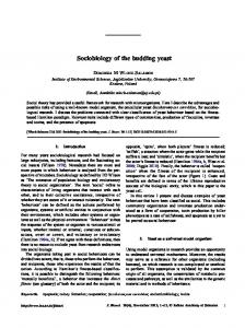
1. Introduction Molecular cell biology describes how cells convert genes into behavior. This description includes how a cell creates proteins from genes, how those proteins interact, and how networks of interacting proteins determine physiological characteristics of the cell. The central biological question addressed here is how protein interactions regulate the cell cycle of budding yeast (Saccharomyces cerevisiae). The budding yeast cell cycle consists of four phases (see Figure 1), with cell division occurring in the final

SIMULATION, Vol. 83, Issue 7, July 2007 497–514 c 2007 The Society for Modeling and Simulation International 1

DOI: 10.1177/0037549707085075 Figures appear in color online: http://sim.sagepub.com

phase. A newborn cell starts in G1 phase (unreplicated DNA), during which time it grows to a sufficiently large size to warrant a new round of DNA synthesis (S phase). After DNA synthesis has completed, the cell passes briefly through G2 phase (replicated DNA) and then enters M phase (mitosis, where the two copies of each DNA molecule are separated and the cell divides, creating two new cells that are in G1 phase). The protein interactions that govern these cell cycle events are modeled using differential equations that describe the rate at which each protein concentration changes. In general, the concentration of protein A, written as [A], changes according to the differential equation d [A] dt

2 synthesis 3 degradation 3 binding 4 dissociation 3 inactivation 4 activation1 Volume 83, Number 7 SIMULATION


497

Panning, Watson, Shaffer, and Tyson

Figure 1. The phases and stages of the cell cycle. The four phases of the cell cycle are shown above the 1ve stages. The events that delineate the cell cycle are at the bottom.

where “synthesis” is the rate at which new protein A molecules are synthesized from amino acids (which depends on the concentration of active messenger RNA molecules for a particular protein), “degradation” is the rate at which protein A is broken down into amino acids and polypeptide fragments (which depends on the activity of specific proteolytic enzymes), “binding” is the rate at which protein A combines with other molecules to form distinct molecular complexes, “dissociation” is the rate at which these complexes break apart, “inactivation” is the rate at which certain post-translational modifications (e.g., phosphorylation) of protein A are made, and “activation” is the rate at which these modifications are reversed (e.g., dephosphorylation). Each of these rates is itself a function of the concentrations of the interacting species in the network. For example, 1 2 synthesis 2 k1 transcription factor 1 1 2 degradation 2 k2 proteolytic enzyme [A] 1 binding 2 k3 [A] [B] 1 where B is a binding partner1 dissociation 2 k4 [AB] 1 inactivation 2

A simple example illustrating the spirit of the modelling approach in this paper follows. A rudimentary reaction network for the frog egg cell cycle [22] results in the three ordinary differential equations dM dt

2 34 d5 31 3 D5 4 4 d55 D53C T 3 M5 3 34 65 31 3 W 5 4 4 655 W 5M1 3

dD dt

2 4d

dW dt

2 46

3

4

7 6 31 3 W 5 3M W 4 K m6 4 W K m6r 4 31 3 W 5

1 4 1

where M, D, and W are normalized protein concentrations, the K s, 7s, and 4s are rate constants, and the constant C T is total (normalized) cyclin. For C T above some threshold C A , the cell enters mitosis and cycles. Finding this threshold and the periodic solution defining the cell cycle could be modelled by the system of constraints 0 8 9 8 t1 1

k5 [kinase] [A] 1 J5 4 [A]

1 21 2 k6 phosphatase A p 1 2 activation 2 1 J6 4 A p

M3t1 5 2

M3t1 4 9 5 2 M3t1 4 29 51

dM dt 3t1 5

dM dM 3t1 4 9 5 2 3t1 4 29 51 dt dt

CA where A p is the phosphorylated form of A2 In these rate laws, the ks are rate constants and the J s are Michaelis constants. Other differential equations must be used to determine the temporal dynamics of the concentrations of the “transcription factor,” “proteolytic enzyme,” “kinase,” etc. 498 SIMULATION

7d D M31 3 D5 3 K md 4 31 3 D5 K mdr 4 D

2

8 CT 1

where the variables would be a time t1 , a period 9 , and a threshold C A . The budding yeast cell cycle model [7] consists of 36 such differential equations for two classes of variables: regulatory proteins and physiological “flags.” The regulatory proteins are triggers for specific events of the budding yeast cell cycle: Cln2 triggers budding, Clb5 triggers DNA synthesis, Clb2 drives cells into mitosis, and Esp1

Volume 83, Number 7


A MATHEMATICAL PROGRAMMING FORMULATION FOR THE BUDDING YEAST CELL CYCLE

drives cells out of mitosis and back to G1. The physiological “flags” are dummy variables that track the strength of these trigger proteins. For example, “BUD” is an integral of the activity of Cln21 when BUD 2 1, a new bud is initiated. “ORI,” an integral of [Clb5], represents the state of “origins of replication.” When ORI 2 1 (this state is called “fired” origins), DNA synthesis is initiated1 at cell division, when [Clb2] 4 [Clb5] drops below a threshold level, ORI is reset to zero (called “licensed” origins). Finally, “SPN” represents the alignment of replicated chromosomes on the mitotic spindle. SPN is driven by Clb2 activity1 i.e., SPN is an integral of [Clb2]. In the budding yeast model there are 143 rate constant parameters (ks, J s, etc.). In some cases, these parameters can be calculated directly from laboratory experiments (e.g., apparent protein half-lives), but most parameters are difficult to obtain directly from experimentation. Normally, modelers determine the remaining parameters by making educated guesses, solving the differential equations numerically, comparing the simulation results with laboratory data, and then refining their guesses. (Modelers call this process “parameter twiddling” [2].) For the budding yeast cell cycle, the laboratory data consists of observed phenotypes of more than 100 mutant yeast strains constructed by disabling and/or over-expressing the genes that encode the proteins of the regulatory network. Although parameter twiddling is extremely tedious, it was used to obtain a parameter vector (s1 , s2 1 2 2 2 1 s143 ) for which the model’s predictions are consistent with almost all of the budding yeast mutants being modeled. Obviously, the modelers would prefer a method that allows them to spend more time improving the equations and less time tuning parameters. In addition, a person can only keep track of a few parameters at one time, which makes it easy for him or her to unwittingly miss a portion of the parameter space. For these reasons, modelers would prefer to use a tool that determines “good” parameters automatically, quickly, and accurately. The current approach to this parameter estimation (nonlinear regression) problem is to assign a penalty to every discrepancy between the ordinary differential equation (ODE) model’s predictions and experimental data, using all available mutant data, and then do an unconstrained (or simple bound constrained) minimization of this penalty function over the ODE parameter space ([6], [8], [18], [21]). Due to the qualitative nature of the experimental data (Section 2), some of these penalties are discrete and this penalty function is inherently discontinuous, while the ODE solution is a smooth function of the ODE parameters. Beyond the fact that discontinuous objective functions are difficult to minimize, either locally or globally, this penalty approach has deeper flaws. Biologists do not agree on what the penalty should be for a particular discrepancy, or even on which discrepancies should be penalized. This paper takes a quite different approach to parameter estimation. The idea is to describe the mutant data as

a system of smooth nonlinear inequalities derived from the (smooth) ODE model output and cell biology knowledge. These inequalities should be generally accepted by cell biologists, even though some of the details may be debatable. An ODE parameter vector that satisfies all of the inequalities thus defines an acceptable model, and is a feasible solution of the system of inequalities. The proposed approach to parameter estimation is to solve a feasibility problem defined by a system of smooth (continuous, piecewise C 6 ) inequalities. One could surmise that what really is desired is the “most interior” point, defined by, e.g., constraint margins. The situation is not so simple, though, since a cell’s viability is robust with respect to environmental variations, and therefore it is really the “most robust” feasible point that is sought. Modeling such biological robustness is another research topic. The paper is organized as follows. After some definitions, Section 2 provides the necessary biology background. As a point of reference, Section 3 describes the penalty function model, and reports parallel computing results obtained on the 2200 processor System X. Section 4 presents the inequality models for all the mutants, the heart of the paper. Some preliminary numerical results for the model are given in Section 5, but an attempt to solve the full model (with approximately 11,500 constraints and 4,000 variables) is a major long term project.

2. Observed and Predicted Phenotypes Experimental biologists have studied many budding yeast mutants to learn about the cell cycle regulatory system. Of these mutants, 115 were chosen to model (see Appendix A). A model of budding yeast can be considered acceptable only if it is able to duplicate the behavior of most of these mutants. (It would be too much to expect a model to account for all the “observations” because of lingering uncertainties about the reaction network and inevitable mistakes in phenotyping mutants.) When the model is used to simulate a mutant, the parameter vector can be changed only in ways that are dictated by the genetic changes in the mutant. Consider the hypothetical proteins A and B presented in the previous section: if a mutant has a modified form of B that does not bind to A, then in the parameter vector for that mutant, k3 would be set to zero and all the other parameters would be kept at the wild type values. The observed phenotype refers to the phenotype that was recorded in a laboratory experiment. The predicted phenotype refers to the phenotype that the mathematical model (with its associated parameters) predicts. The wild type is the normal strain of an organism. The mutant strains have genetic changes that make them behave differently from the wild type in some way. When comparing the model to the experimental data, it is important to realize that much of the data from laboratory experiments is qualitative. Such data is of the form Volume 83, Number 7 SIMULATION


499


“the cell is viable but considerably larger than wild type cells” or “the cell arrests in G1 phase and eventually dies.” The quantitative data that is available (e.g., duration of G1 phase, cell mass at division) is generally imprecise. With all these uncertainties, there may be many, clustered parameter vectors that allow the model to reproduce the experimental data sufficiently well. What matters for the model here is the structure of the cell cycle regulatory pathways, not the details of the biochemistry.

bud), then the predicted phenotype of that mutant must exhibit the same behavior. It is possible for a cell to complete all of the checkpoints in the first cycle and then become arrested somewhere in the second cycle. If a cell has this type of observed phenotype, then a correct model must predict the same number of cycles before arresting in the same manner. If the observed cell has a viable phenotype, then the model must predict a viable cell with a similar G1-phase length, and a similar mass at division.

2.1 Rules of Viability

2.2 Initial Conditions

To compare solutions of the differential equations with experimental data, it is necessary to predict cell cycle properties from a simulation of regulatory protein dynamics. Viability is determined by four rules:

In the experimental data set, many of the mutations are conditional, that is, the mutant cells when grown under “normal” conditions (say, glucose medium at room temperature) behave like wild-type cells, but when grown under “restrictive” conditions (say, galactose medium or elevated temperature) the cells express the genetic mutation and the aberrant phenotype. To model this situation at sample points in parameter space, start a “wild-type” simulation from arbitrary (but reasonable) initial conditions and integrate the differential equations for two full cycles, in order to wash out any effects of the initial conditions. Then record the state of the control system just after [Clb2] 4 [Clb5] falls through K ez2 at the beginning of the third cycle. These recorded values are used as initial conditions for simulating a steady state wild-type cell and for simulating each of the mutants.

1. The modeled cell must execute the following events in order, or else the modeled cell is considered inviable: (a) DNA licensed for replication (modeled by a drop in [Clb2] 4 [Clb5]below K ez2 , which resets [ORI] to zero)1 (b) start of DNA synthesis (due to a subsequent rise in [Clb2] 4 [Clb5], causing [ORI] to increase above one), signaling the end of G1 phase, before a wild-type cell in the same medium would divide twice1 (c) alignment of DNA copies (due to a rise in [Clb2], causing [SPN] to increase above one) while [Esp1] is less than 0.11 (d) separation of DNA copies (modeled by [Esp1] increasing above 0.1, due to Pds1 proteolysis at anaphase)1 (e) cellular division (modeled by [Clb2] dropping below a threshold K ez ), which resets [BUD] and [SPN] to zero. 2. The cell is inviable if division occurs in an “unbudded cell” (i.e., if [BUD] does not reach the value 0.8 before event (e) occurs). 3. The cell cycle should be stable, i.e., the squared relative differences of the masses and G1 phase durations in the last two simulated cycles should both be less than 0.05. 4. Lastly, the modeled cell is considered inviable if cell mass at division is greater than four times or less than one-fourth times the steady-state mass at division of the wild type in the same medium. If the observed phenotype for a mutant does not complete one of the checkpoints (e.g., the mutant cells do not 500 SIMULATION

3. Nonsmooth Penalty Function Formulation This section describes a typical deviation (model prediction minus observed system response) based formulation of the parameter identification problem as the unconstrained (or at most simple bound constrained) minimization of a nonsmooth objective function. Numerical results using 1024 processors are presented for two different applicable optimization algorithms. Since these runs required many hours on 1024 processors, the need for high performance computing for the smooth inequality formulation in the next section should be clear. The objective function takes the observed phenotype and predicted phenotype for all of the mutants and computes a nonnegative score. Zero indicates a perfect match and larger numbers indicate increasingly worse matches. The ensuing discussion uses the symbol O for observed phenotype values and P for predicted phenotype values. A budding yeast phenotype for a single mutant is represented by a six-tuple (4, g, m, a, t, c), where the viability 4 7 8viable, inviable9, the real number g 0 is the steady state length of the G1 phase, the real number m 0 is the steady state mass at division, the stage when arrest occurred is a 7 8unlicensed1 licensed1 fired1 aligned1 separated9 1

Volume 83, Number 7



the positive integer t is the arrest type, and the nonnegative integer c is the number of successful cycles completed. The observed and predicted phenotypes are written O 2 3O4 1 Og 1 Om 1 Oa 1 Ot 1 Oc 5 and P 2 3P4 1 Pg 1 Pm 1 Pa 1 Pt 1 Pc 5, respectively. Arrest types cannot be compared unless the stage of arrest is the same for both phenotypes. In what follows, the s and s are constants defined in Table 1. The rating function, R, compares the observed and predicted phenotypes for a mutant. This rating function is a modified version of the one developed by N. Allen et al. [3]1 the only difference is that if O4 or P4 is missing, then R3O1 P5 2 4 . The rating function is split into four cases depending on the viability of the observed and predicted phenotypes. If O4 2 inviable, P4 2 viable, and Oc is missing, then R3O1 P5 2 4 , the same as if Oc 2 0. Otherwise, if a needed classifier is missing, the term is simply dropped and does not contribute to the objective function. In the case that classifiers are missing, this allows the objective function value to be at or near zero when viability is in agreement between the phenotypes, and forces larger objective function values when viability is not in agreement. The rating function R3O1 P5 when all classifiers are present is given by 5 O 62 4 3 ln Pmm Og 3 Pg 2 4 m

1 g

g m if O4 2 viable and P4 2 viable, by 1 1 4

1 4 Pc if O4 2 viable and P4 2 inviable, by 4 3 Oc 3 Pc 2

O1P 4 c

1 c

Table 1. Constants used in objective function. Symbol

De1nition

Value

g g m m a t c c 4

G1 length weight

1.0

if O4 2 inviable and P4 2 viable, where is a real valued discrete function, used to assess a penalty for the arrest stage and type, given by 7 a 1 if Oa 2 Pa 1 8 8 9 t 1 if Oa 2 Pa and Ot 2 Pt 1

O1P 2 8 8

01 if Oa 2 Pa and Ot 2 Pt 2 The rating function is tuned by parameters to allow the modeler to adjust the relative importance of classifiers. The parameters given by Table 1 were set so that a rating of around ten indicates a critical error in the model’s prediction of a phenotype.

10.0

Mass at division weight

1.0

Mass at division scale

ln 2

Arrest stage weight

10.0

Arrest type weight

5.0

Cycle count weight

10.0

Cycle count scale

1.0

Viability weight

40.0

Denote the real numbers by 1, the nonnegative integers 801 11 21 2 2 29 by 24 , and the integers by 2. Let 3 2 341 g1 m1 a1 t1 c5 2 8viable1 inviable9 301 652

8unlicensed1 licensed1 fired1 aligned1 separated9

811 2 2 2 1 109 24 be the space of all budding yeast phenotypes and let the domain of the objective function be the box 2 8x 7 1143 : si u i xi si u i 1

i 2 11 2 2 2 1 14391

where u 7 1 are positive scale factors reflecting modelers’ knowledge about the rate constants, and s 7 1143 is the modeler’s best guess point. Let T j : 3 simulate the jth mutant with the parameters x1 1 2 2 2 1 x143 and compute the phenotype. Then the objective function f : [01 6) is defined by 143

if O4 2 inviable and P4 2 inviable, and by 1 1 4

1 4 Oc

G1 length scale

f 3x5 2

Nm

j R3O j 1 T j 3x551

j21

where Nm is the number of mutant experiments, and i 7 811 49 is a weight that indicates whether the ith mutant is of normal or high importance. The objective function value at the biologists’ best previously known point [7] is 433. Two algorithms that show promise for optimizing the discontinuous objective function are briefly described next. Consider the problem of minimizing f : B 1, where B 2 [l1 u] 1n is a box. 3.1 DIRECT The DIRECT (Dividing Rectangles) global minimization algorithm [14] requires the objective function to be Lipschitz continuous to guarantee convergence. Even though Volume 83, Number 7 SIMULATION


501


the objective function used here is discontinuous, the DIRECT algorithm seems to be an efficient and reasonable deterministic sampling strategy worth trying. The DIRECT algorithm is one of a class of deterministic direct search algorithms that does not require gradients. It works by iteratively dividing the search domain into boxes that have exactly one function value at the box’s center. In each iteration, the algorithm determines which boxes are most likely to contain a better point than the current minimum point—these boxes are called “potentially optimal”. It then subdivides the potentially optimal boxes along their longest dimensions. Intuitively, a box is considered potentially optimal if it has the potentially best function value for a given Lipschitz constant. For an illustration of how the DIRECT algorithm searches the domain on an example problem, see [20]. Both serial [10] and parallel ([11]–[13]) versions of DIRECT have been described in the literature. 3.2 MADS A MADS (Mesh Adaptive Direct Search) algorithm, as defined by Audet and Dennis [5], minimizes a nonsmooth function f : 1n 1 8469 under general constraints x 7 1n , 2 . If 2 1n , the algorithm works with f , which is equal to f on and 46 outside . Using f in lieu of f is called a “barrier” approach to handling arbitrary constraints x 7 . In each iteration, a MADS algorithm evaluates the objective function f at a finite number of trial points. Central to these algorithms is the concept of a mesh, which is a discrete set of points in 1n . Every previous trial point must lie on the current mesh, and in each iteration the algorithm may only generate new trial points on the current mesh. This is not as restrictive as it might sound because the algorithm changes the mesh after each iteration (with the restriction that at iteration k all previously evaluated points Sk remain in the new mesh). Each iteration of a MADS algorithm consists of two steps: the SEARCH step and the POLL step. The SEARCH step may evaluate f at any finite number of mesh points. At which mesh points f is evaluated depends on the precise MADS algorithm in use. If the SEARCH step fails to find a mesh point at which f is less than minx7Sk f 3x5, then the algorithm performs the POLL step by generating and evaluating f at new trial points around the current incumbent solution xk , where f 3xk 5 2 minx7Sk f 3x5. The p poll size parameterk limits the distance between xk and the new trial points. The set of new trial points is called a frame, and x k is called the frame center. The algorithm evaluates f at points in the frame Pk until it encounters an improved point x ( f 3x 5 8 f 3xk 5) or it has evaluated f at all of the points in Pk . After the algorithm has executed the SEARCH step and (conditionally) the POLL step, it sets the mesh size and p poll size parameters, m k41 and k41 , for the next iteration. 502 SIMULATION

p

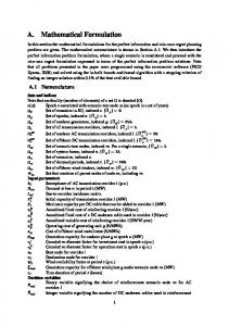
Exactly how m k41 and k41 are generated is determined by the individual algorithm in use. More precise descriptions of the MADS class of algorithms with examples can be found in [5] or [18]. 3.3 Parallel Optimization Results All computation took place on System X, a cluster of 1100 dual-processor Mac G5 nodes. NOMAD is a C++ implementation of the MADS class of algorithms. To take advantage of System X, NOMAD’s implementation of the POLL step was parallelized using a master/worker paradigm. The master ran the MADS algorithm as presented and sent requests to the workers whenever objective function values were needed. NOMAD, started from the modeler’s best point s, evaluated the objective function 135,000 times over 813 iterations using 128 processors, converging at a point for which the objective function value was 299 (this point correctly models all but ten of the mutants). pVTDirect [11] is a parallel implementation of DIRECT written in Fortran 95. While the DIRECT algorithm does not have a traditional “starting point”, the first sample in each subdomain is always taken at the center of the subdomain bounding box. For this problem, the bounding box was designed so that the modeler’s best point would be at the center and therefore would be evaluated before any other points. pVTDirect (with only one subdomain) ran for 473 iterations using 1024 processors and evaluated the objective function 1.5 million times, finding a point at which the objective function value was 212 (this point correctly models all but eight of the mutants). Figure 2 shows the progress that each program was able to make in minimizing the objective function. While NOMAD was able to quickly find a better point than the modeler’s best point, pVTDirect was eventually able to find an even lower point. This is expected behavior because NOMAD is designed for local optimization and pVTDirect is designed for global optimization, so NOMAD quickly found a nearby local minimum and stopped, but pVTDirect explored the parameter space and eventually found a better minimum. In a later run, NOMAD was started from pVTDirect’s lowest point, but NOMAD was unable to make any further progress. After looking at Figure 2, it is tempting to believe that pVTDirect could have been stopped earlier (for instance, after 200,000 evaluations), and NOMAD started at pVTDirect’s last best point could have found a point at which the objective function value was 212 or less. To test this, NOMAD was started at the best point at the 54th, 157th, and 239th iterations of pVTDirect. These points correspond to the beginning, middle, and end of the second-lowest plateau in Figure 2. As shown in Figure 3, NOMAD started from the middle point converged to a point at which the objective function value was 210. However, the NOMAD runs started at the beginning and

Volume 83, Number 7



Figure 2. The objective function value at the best point found versus the number of evaluations for MADS and DIRECT.

Figure 3. The performance of NOMAD when started from the best point at pVTDirect’s 54th, 157th, and 239th iterations. The plots are shown as if the NOMAD runs started as soon as the respective pVTDirect iterations completed.

end plateau points converge to worse points than pVTDirect’s best point. These four extra NOMAD runs (including the one starting from pVTDirect’s best point) show that an algorithm for improving intermediate results from pVTDirect is not so clear. Finally, recall that f 3x5 0 means some mutant experimental data is not being matched, i.e., the parameters

found by DIRECT and MADS do not fully explain all the data. These results motivated the smooth inequality formulation given next.

Volume 83, Number 7 SIMULATION


503


4. Formulation of Conditions as a Nonlinear System of Inequalities For each phenotype, this section presents a system of constraints that will be satisfied if and only if the simulation predicts the same phenotype. The constraints are written 1 2 using as much biological notation as possible, so Esp1 3t6 5 refers to the concentration of the protein Esp1 at the time t6 . The constraints include time variables ti where i is a positive integer1 although these variables are not part of the model, they must still be found by the parameter estimator. In the constraints, there are several constants which are set as follows: 2 0205, G 1 2 20, and

M 2 124.

4.1 Viable Phenotype Constraints The constraints for a viable cell to go through one cycle are listed below, with annotations denoted by parantheses. t1 8 t2 8 t3 8 t4 8 t5 8 t6 8 t8 1 (1) t3 3 t1 8 t6 1

(2)

t2 8 t7 8 t8 1 G 1 3 G 1 8 t3 3 t0 8 G 1 4 G 1 1

(3)

t1 t t2

K ez2 [Clb2] 3t2 4 5

max [ORI] 3t5 8 1 8 [ORI] 3t3 4 51

t2 4 t t3

max [SPN] 3t5 8 1 8 [SPN] 3t5 51

t1 t t4

1 2 1 2 max Esp1 3t5 8 021 8 Esp1 3t6 51

t4 t t5

[BUD] 3t7 5 0281

max [mass] 3t5 8 4m 6 1

t1 t t8 3

42 8 0205

and

3t3473N 325 3t1473N 325 533t3473N 315 3t1473N 315 5 3t3473N 325 3t1473N 325 5

2

8 02051

where N is the total number of cycles. 4.2 Phenotypes for pds1 Mutants (6) (7) (8)

The pds1 mutants are incapable of synthesizing Esp1, but some of these mutants still manage to separate the DNA copies. It is suspected that these mutants use a different mechanism to separate the DNA, but that mechanism is not included in this model. So for the purposes of this model, pds1 mutants are not required to meet viability rule 1(d), and the corresponding constraints should be omitted when evaluating mutants 61, 62, 66, 67, 71, and 113 in Appendix A.

(10) 4.3 Inviable Phenotype Constraints (11)

M 3 M 8 [mass] 3t8 3 5 8 M 4 M 2 (12)

504 SIMULATION

[mass] 3t8473N 325 5 3 [mass] 3t8473N 315 5 [mass] 3t8473N 325 5

(5)

(9)

[Clb2] 3t8 3 5 K ez [Clb2] 3t8 51

3

(4)

min 3[Clb2] 3t5 4 [Clb5] 3t55

4 [Clb5] 3t2 4 51

(1) These strict inequalities ensure the correct temporal ordering of the events defined by the times ti . (2) [ORI] must rise above one before a wild type cell would divide twice in the same medium (e.g., glucose or galactose)1 t6 is set to the amount of time a simulated wild type cell takes to divide twice with the same biological parameters. (3) t7 (which marks [BUD] rising above one) simply has to occur any time between t2 and t8 . (4) G 1 is the length of the G1-phase, as observed in experiments. This ensures that the simulated cell is within a predefined distance G 1 of the observed value. (5) [Clb2] 4 [Clb5] drops, satisfying viability rule 1(a). (6) [ORI] rises, satisfying rule 1(b). (7) [SPN] rises, satisfying rule 1(c). (8) [Esp1] rises, satisfying rule 1(d). (9) [BUD] rises, satisfying rule 2. (10) [Clb2] drops, satisfying rule 1(e). (11) Mass is always less than four times the mass of the wild type in the same medium1 m 6 is the mass of a simulated wild type cell with the same biological parameters. (12) M is the observed mass at division. A cell that meets the above constraints is viable for one cycle. For the first cycle, remember that the starting conditions are just after [Clb2] 4 [Clb5] dropped through K ez2 , so the fifth constraint must be omitted. For the rest of the cycles, repeat the constraints with variables t1473n315 , t2473n315 , 2 2 2, t8473n315 for cycle n. Note that the last time of the previous cycle is the first time in the current cycle. To enforce the stability requirements, add the constraints

A cell that fulfills the above constraints is considered viable. Some of the mutants have an observed phenotype of inviable, so their constraints will be different. The constraints for an inviable mutant are determined by when

Volume 83, Number 7



max [SPN] 3t5 8 11

and how the cell arrests. There are four major types of arrest stages: G1 arrest, metaphase arrest, G2 arrest, and telophase arrest. The following subsections present the inequality constraints for each of these arrest types.

0 t t4

max [mass] 3t5 4m 6 2

0 t t4

4.4 G1 Arrest

4.6 Metaphase Arrest

In terms of the model, a G1 arrest means that none of [ORI], [SPN], or [BUD] should rise to one before the cell cycle is considered arrested. Whether or not [Clb2] 4 [Clb5] drops below K ez has no effect on whether the cell is G1 arrested, so it is not mentioned in the constraints. A cell arrests in G1 either because its mass has become greater than 4m 6 (see viability rule 4) or because t6 time has passed (see checkpoint 1(b)). Constraints for a G1 arrested mutant are thus

If a cell is arrested in metaphase, its chromosomes are aligned on its spindles (i.e., the [SPN] checkpoint must be reached) but the chromosomes have not separated (i.e., Esp1 has not activated). Metaphase arrested cells may be budded or unbudded. This means that the following constraints must be met. t1 t3 3 t1

max8t1 3 t6 1 max [mass] 3t5 3 4m 6 9 01

8 t2 8 t3 8 t4 8 t5 8 t6 1 8 t6 1

0 t t1

min 3[Clb2] 3t5 4 [Clb5] 3t55

t1 t t2

max [ORI] 3t5 8 11

0 t t1

max [SPN] 3t5 8 11

4 [Clb5] 3t2 4 51

0 t t1

max [BUD] 3t5 8 12

0 t t1

The first inequality ensures that t1 is a time after the cell has arrested. Specifically, the quantity t1 3 t6 will be greater than zero if a wild type cell could divide twice before t1 . Similarly, the quantity max0 t t1 [mass] 3t5 3 4m 6 will be greater than zero if the cell has grown to a mass greater than 4m 6 before t1 . The maximum of these quantities is used because violating any of the viability rules causes a cell to be arrested.

max [ORI] 3t5 8 1 8 [ORI] 3t3 4 51

t2 4 t t3

max [SPN] 3t5 8 1 8 [SPN] 3t5 51

t1 t t4

1 2 max Esp1 3t5 8 0211

t4 t t5

max [mass] 3t5 4m 6 2

0 t t6

4.7 Telophase Arrest

4.5 G2 Arrest For a cell to be arrested in G2, it must execute the first two checkpoints of a viable cell, but [SPN] must stay low. t1 t3 3 t1

8 t2 8 t3 8 t4 1 8 t6 1 min 3[Clb2] 3t5 4 [Clb5] 3t55

t1 t t2

K ez2 [Clb2] 3t2 4 5

4 [Clb5] 3t2 4 51 max [ORI] 3t5 8 1 8 [ORI] 3t3 4 51

t2 4 t t3

K ez2 [Clb2] 3t2 4 5

While the G1 phase is the earliest a cell can be arrested, telophase is the latest a cell can become arrested. A telophase arrested cell must complete all of the checkpoints except that [Clb2] can not drop below K ez before the cell arrests. The first eight constraints for such a cell would be the same as the constraints for a viable cell. The ninth constraint would be removed, and the tenth constraint would be changed to max [Clb2] 3t5 8 K ez 8

t2 4 t t7

min

t7 4 t t8

[Clb2] 3t51

with the additional constraints t1

8 t7 8 t8 1

[mass] 3t8 5 4m 6 2 Volume 83, Number 7 SIMULATION


505


4.8 Evaluating All of the Mutants

Section 3). There is a similar algorithm for the telophase arrested phenotype.

As described earlier, a parameter vector must satisfy all of the constraints for all of the mutants before it can be considered feasible. Each mutant requires a separate simulation and will have its own set of time variables derived from its concentrations’ trajectories. The mutants are numbered as in Appendix A, so the time for the ith mutant will be t 8i9 . Also, because each mutant modifies the parameter vector slightly, the concentration of a substance at a specific time will vary among the mutants. Rather than explicitly specify which parameter vector is being used, the superscript of the time will indicate the parameter vector being used. For instance, mutant 13 is a G1 arrested mutant, so its constraints would be 8139

max8t1

3 t6 1

max

8139 0 t 8139 t1

[mass] 3t 8139 5 3 4m 6 9 01 max

[ORI] 3t 8139 5 8 11

max

[SPN] 3t 8139 5 8 11

max

[BUD] 3t 8139 5 8 12

8139 0 t 8139 t1

8139 0 t 8139 t1

8139 0 t 8139 t1

5. Biological Results To test this formulation, the constraints for the telophase arrest and viable phenotypes were evaluated at two parameter vectors. The pds1 mutants were excluded from this test, leaving 61 mutants with an observed phenotype of viable and 15 mutants with an observed phenotype of telophase arrested. The first parameter vector used the best manually obtained biological parameters [7], and the second vector used the best biological parameters found using optimization algorithms on a penalty function formulation of the problem [18]. For both vectors, the time parameters were found using an algorithm that examines the ODE model simulation time series output and picks sensible values. In one pass through the simulation time series output, this algorithm attempts to pick the time variables so that they are in the proper order, and if possible, the constraints are satisfied. During the simulation, the algorithm keeps track of the maximum and minimum values for the model variables in the constraints (e.g., [BUD], [SPN]). When an event (cf. Section 2.1) occurs, the algorithm sets the respective time variables and then checks to see if all of the earlier time variables have been set. If there are earlier time variables that have not been set, the algorithm attempts to set each of them to a time that maintains the ordering of the variables and minimizes the violation of the constraints. A more formal description of this algorithm (for the viable phenotype) is given below ( comes from the beginning of 506 SIMULATION

check_*: flags for checking earlier events o: offset into the time parameters n c : number of cycles completed reset_cycle: flag for resetting best times s: maximum time that a previous event can be set to t: current time t f : end of the simulation time tb : best time for [BUD] rising tc : best time for 1[Clb2]24 [Clb5] dropping te : best time for Esp1 rising tr : best time for [ORI] rising ts : best time for [SPN] rising t :2 01 n c :2 01 o :2 11 s :2 01 tc :2 01 tr :2 01 ts :2 01 te :2 01 tb :2 0 while 3t 8 t f 5 do check_Clb2_Clb5 := false1 check_ORI := false1 check_ORI := false1 check_SPN := false check_Esp1 := false1 check_BUD := false1 reset_cycle := false if (n c 1) then o:2 8 4 3n c 3 15 7 else o:2 1 end if Advance t to the next time in the ODE simulation time series output. if ([Clb2] 4 [Clb5] dropped through K ez2 ) then to41 :2 t 3 21 tr :2 311 ts :2 311 te :2 31 elseif ([ORI] rose through one) then to42 :2 t 3 21 s:2 to42 3 1 ts :2 311 te :2 311 check_Clb2_Clb5 := true elseif ([SPN] rose through one) then to43 :2 t 3 1 to44 :2 t 4 1 s:2 to43 3 1 te :2 311 := true 1 check_ORI 2 elseif ( Esp1 rose through 0.1) then to45 :2 t 4 1 s:2 to45 3 1 check_SPN := true elseif ([BUD] rose through one) then to46 :2 t 4 elseif ([Clb2] rose through K ez ) then to47 :2 t 3 21 n c :2 n c 4 11 s:2 to47 3 check_Esp1 := true1 check_BUD := true1 reset_cycle := true end if if (check_BUD 2 true and to46 has not been set) then if ([BUD] 3s5 8 [BUD] 3tb 5) then to46 :2 tb else to46 :2 s end if end if if (check_Esp1 2 true and to45 has not been set) then

Volume 83, Number 7



1 2 1 2 if ( Esp1 3s5 8 Esp1 3te 5) then to45 :2 te else to45 :2 s end if check_SPN := true end if s:2 to45 3 if (check_SPN 2 true and to44 has not been set) then if ([SPN] 3s5 8 [SPN] 3ts 5) then to43 :2 ts 3 1 to44 :2 ts 4 else to43 :2 s 3 1 to44 :2 s 4 end if check_ORI := true end if s:2 to43 3 if (check_ORI 2 true and to42 has not been set) then if ([ORI] 3s5 8 [ORI] 3tr 5) then to42 :2 tr else to42 :2 s end if check_Clb2_Clb5 := true s:2 to42 3 if (check_Clb2_Clb5 2 true and to41 has not been set) then if ([Clb2] 3s5 4 [Clb5] 3s5 [Clb2] 3tc 5 4 [Clb5] 3tc 5) then to41 :2 tc else to41 :2 s end if end if if (reset_cycle 2 true) then tc :2 311 tr :2 311 ts :2 311 te :2 311 tb :2 31 end if if ([Clb2] 3t54[Clb5] 3t5 8 [Clb2] 3tc 54[Clb5] 3tc 5 or tc 8 0) then tc :2 t end if if ([ORI] 3t5 [ORI] 3tr 5 or tc 8 0) then tr :2 t end if if ([SPN] 3t5 [SPN] 3ts 5 or tc 8 0) then ts :2 t end1 if 2 1 2 if ( Esp1 3t5 Esp1 3te 5 or tc 8 0) then te :2 t end if if ([BUD] 3t5 [BUD] 3tb 5 or tc 8 0) then tb :2 t end if end while

Table 2. The numbering of the viable constraints for Tables 4, 5, 6, and 7. Index

Constraint

1

10

t1 8 t2 t2 8 t3 t3 8 t4 t4 8 t5 t5 8 t6 t1 8 t7 t7 8 t8 t6 8 t8 t3 3 t1 8 t6 t3 3 t0 3 G 1 8 G 1

11

G1 stability constraint

12

24

mint1 t t2 3[Clb2] 3t5 4 [Clb5] 3t55 K ez2 K ez2 [Clb2] 3t2 4 5 4 [Clb5] 3t2 4 5 maxt2 4 t t3 [ORI] 3t5 8 1 1 8 [ORI] 3t3 4 5 maxt1 t t4 [SPN] 3t5 8 1 1 8 [SPN]13t5 5 2 maxt4 t t5 Esp1 3t5 8 021 1 2 021 8 Esp1 3t6 5 [BUD] 3t7 5 1 [Clb2] 3t8 3 5 K ez K ez [Clb2] 3t8 5 maxt1 t t8 3 [mass] 3t5 8 4m 6 [mass] 3t8 3 5m 6 3 M 8 m

25

Mass stability constraint

2 3 4 5 6 7 8 9

13 14 15 16 17 18 19 20 21 22 23

For conciseness, the violated constraints for viable mutants are listed as “Cx-Ny”, where x indicates the cycle in which the violation occurred, and y is an index into Table 2 that indicates which constraint was violated. The violated constraints for telophase-arrested mutants are listed as “Ny”, where y is an index into Table 3. The results of evaluating the viable constraints on all of the mutants with an observed phenotype are shown in Tables 4, 5, 6, and 7. Tables 4 and 5 show the mutants that satisfied and did not satisfy the constraints, respectively, when the manually obtained biological parameters were used. Tables 6 and 7 show the same for the mathematically optimized biological parameters. A parallel direct search algorithm [15] applied to the penalty function formulation used over 10,000 CPU hours on 400 processors of a 2200 processor supercomputer (1100 Apple G5 Xserve nodes, Infiniband network). The full inequality formulation for all mutants would have approximately 11,500 constraints (sum of constraints per phenotype accounting for multiple cycles) and 4000 variVolume 83, Number 7 SIMULATION


507


Table 3. The numbering of the telophase arrest constraints for Tables 4, 5, 6, and 7. Index

Constraint

1

t1 8 t2 t2 8 t3 t3 8 t4 t4 8 t5 t5 8 t6 t1 8 t7 t7 8 t8 maxt2 4 t t3 [ORI] 3t5 8 1 1 8 [ORI] 3t3 4 5 maxt1 t t4 [SPN] 3t5 8 1 1 8 [SPN]13t5 5 2 maxt4 t t5 Esp1 3t5 8 021 1 2 021 8 Esp1 3t6 5 maxt1 4 t t7 [Clb2] 3t5 8 K ez K ez 8 mint7 4 t t8 [Clb2] 3t5 [mass] 3t8 5 4m 6

2 3 4 5 6 7 8 9 10 11 12 13 14 15 16

Table 4. Mutants that had no violated constraints, manually obtained parameters.

Wild type in glucose Wild type in galactose cln1 cln2 GAL-CLN2 cln1 cln2 cln1 cln2 sic1 cln1 cln2 cdh1 cln3 bck2 Multi-copy BCK2 cln3 bck2 GAL-CLN2 cln1 cln2 cln1 cln2 cln3 GAL-CLN2 cln1 cln2 cln3 GAL-CLN3 cln1 cln2 cln3 sic1 cln1 cln2 cln3 cdh1 cln1 cln2 cln3 multi-copy CLB5 cln1 cln2 cln3 GAL-CLB5 cln1 cln2 cln3 multi-copy BCK2 sic1 GAL-SIC1 GAL-SIC1 GAL-CLN2 cln1 cln2 GAL-SIC1 GAL-CLN2 cln1 cln2 cdh1 sic1 cdh1 GALL-CDC20 cdh1 cdc62-49 508 SIMULATION

Table 4. (continued)

sic1 cdc62-49 GAL-CLB2 Multicopy GAL-CLB2 CLB2-db CLB2-db in galactose CLB2-db multicopy SIC1 CLB2-db GAL-SIC1 CLB2-db clb5 CLB2-db clb5 in galactose clb5 clb6 GAL-CLB5 GAL-CLB5 cdh1 CLB5-db tem1 GAL-TEM1 tem1-ts GAL-CDC15 tem1 net1-ts tem1-ts multicopy CDC14 cdc15 Multicopy CDC15 cdc15 net1-ts cdc15-ts multicopy CDC14 net1-ts GAL-NET1 cdc14-ts GAL-NET1 GAL-CDC14 TAB6-1 cdc15 mad2 bub2 mad2 bub2 APC-A APC-A cdh1 APC-A cdh1 GAL-SIC1 APC-A cdh1 GAL-CDC6 APC-A cdh1 multicopy CDC20 swi5 sic1 cdc62-49 cdh1 GALL-CDC20 APC-A sic1 APC-A GAL-CLB2

ables (almost all of them times t 8i9 j ). One ODE solution and the transforms necessary to match the ODE solution to experimental data take about 17 seconds on a 2.3 GHz G5 processor, so the need for parallel supercomputing is clear. While the nonlinear inequality formulation is definitely large scale, it is well within the range of

Volume 83, Number 7



Table 5. Mutants that had violated constraints, manually obtained parameters.

GAL-CLN2 cln1 cln2 cdh1 GAL-CLN3 cln1 cln2 bck2 cdh1 cdc6 2-49 GAL-CLB2 sic1 GAL-CLB2-db GAL-ESP1 cdc20-ts cdc14-ts GAL-SIC1

TAB6-1 TAB6-1 CLB1 clb2 APC-A cdh1 in galactose

APC-A cdh1 multicopy SIC1 APC-A cdh1 multicopy CDC6

C3-N20, C4-N19, C4-N20, C5-N15, C5-N17, C5-N20, C6-N15, C6-N17, C6-N20, C7-N15, C7-N17, C7-N20, C8-N15, C8-N17, C8-N20 C6-N1, C8-N11, C5-N19, C6-N13, C6-N17, C7-N15, C7-N17, C8-N15, C8-N17 C8-N24 C8-N10 N12, N16 N12 N5, N12 C1-N20, C2-N13, C2-N18, C2-N22, C3-N13, C3-N18, C3-N22, C4-N13, C4-N18, C4-N22, C5-N13, C5-N18, C5-N22, C6-N13, C6-N18, C6-N22, C7-N13, C7-N18, C7-N22, C8-N13, C8-N18, C8-N22 C1-N8 C1-N17, C2-N15, C2-N17, C3-N15, C3-N17, C4-N15, C4-N17, C5-N15, C5-N17, C6-N15, C6-N17, C7-N15, C7-N17, C8-N15, C8-N17 C1-N20, C2-N13, C2-N18, C2-N20, C2-N22, C3-N13, C3-N18, C3-N20, C3-N22, C4-N13, C4-N18, C4-N20, C4-N22, C5-N13, C5-N18, C5-N20, C5-N22, C6-N13, C6-N18, C6-N20, C6-N22, C7-N13, C7-N18, C7-N20, C7-N22, C8-N13, C8-N18, C8-N20, C8-N22 C1-N17, C2-N15, C2-N17 C8-N11, C7-N22, C8-N13, C8-N18, C8-N22

Table 6. (continued) Table 6. Mutants that had no violated constraints, optimized parameters.

Wild type in glucose Wild type in galactose cln1 cln2 GAL-CLN2 cln1 cln2 cln1 cln2 sic1 cln1 cln2 cdh1 GAL-CLN2 cln1 cln2 cdh1 cln3 GAL-CLN3 bck2 Multi-copy BCK2 cln1 cln2 bck2 cln3 bck2 GAL-CLN2 cln1 cln2 cln1 cln2 cln3 GAL-CLN2 cln1 cln2 cln3 GAL-CLN3 cln1 cln2 cln3 sic1 cln1 cln2 cln3 cdh1 cln1 cln2 cln3 multi-copy CLB5 cln1 cln2 cln3 GAL-CLB5 cln1 cln2 cln3 multi-copy BCK2 sic1 GAL-SIC1 GAL-SIC1 GAL-CLN2 cln1 cln2

GAL-SIC1 GAL-CLN2 cln1 cln2 cdh1 sic1 cdh1 GALL-CDC20 cdh1 cdc62-49 sic1 cdc62-49 GAL-CLB2 Multicopy GAL-CLB2 CLB2-db CLB2-db GAL-SIC1 CLB2-db clb5 CLB2-db clb5 in galactose clb5 clb6 GAL-CLB5 GAL-CLB5 cdh1 CLB5-db tem1 GAL-TEM1 tem1-ts GAL-CDC15 tem1 net1-ts tem1-ts multicopy CDC14 cdc15 Multicopy CDC15 cdc15 net1-ts cdc15-ts multicopy CDC14 GAL-NET1 Volume 83, Number 7 SIMULATION


509


problems being solved in industry. This work demonstrates the reasonableness of the inequality approach to parameter estimation for cell cycle modeling. Mechanically assembling all 11,500 constraints and then solving the feasibility problem will be a major undertaking requiring several man-years of effort and parallel supercomputing to evaluate the constraints, but is surely doable.

Table 6. (continued)

cdc14-ts GAL-NET1 GAL-CDC14 TAB6-1 TAB6-1 cdc15 TAB6-1 CLB1 clb2 mad2 bub2 APC-A APC-A cdh1 APC-A cdh1 in galactose APC-A cdh1 multicopy SIC1 APC-A cdh1 GAL-SIC1 APC-A cdh1 multicopy CDC6 APC-A cdh1 GAL-CDC6 APC-A cdh1 multicopy CDC20 swi5 APC-A sic1 APC-A GAL-CLB2

6. Conclusions

Table 7. The mutants that had violated constraints, optimized parameters.

cdh1 cdc62-49 GAL-CLB2 sic1 CLB2-db in galactose CLB2-db multicopy SIC1 GAL-CLB2-db GAL-ESP1 cdc20-ts net1-ts cdc14-ts GAL-SIC1

mad2 bub2 sic1 cdc62-49 cdh1 GALL-CDC20

510 SIMULATION

C8-N10 N12, N16 N16 C8-N22, C8-N25 N12 N5, N12 C1-N8 C1-N20, C2-N13, C2-N22, C3-N13, C3-N22, C4-N13, C4-N22, C5-N13, C5-N22, C6-N13, C6-N22, C7-N13, C7-N22, C8-N13, C8-N22 C1-N16 C1-N16, C1-N18

C2-N18, C3-N18, C4-N18, C5-N18, C6-N18, C7-N18, C8-N18,

A long-range goal of system biology is to develop efficient tools for fitting quantitative models to available types of experimental data. The cell cycle control system in budding yeast is a representative example of this general problem. The model consists of 36 variable protein levels (described by ordinary differential equations) and 143 kinetic parameters that need to be estimated from the data. The data consists of a hodge-podge of qualitative observations and quantitative measurements on wild-type and mutant cells. The challenge is to determine if there exists a feasible set of kinetic parameters for which the ODEs are consistent with the qualitative phenotypes of the collection of mutants. This problem is formulated as a system of nonlinear inequalities that is satisfied if and only if the model matches all experimental data. The results in Tables 4–7 show that this formulation can accurately compare the simulation results with the experimental data. Using the smooth constraints instead of the discontinuous objective function will make it possible to use mathematical programming algorithms that assume smooth functions. Note that no 143-dimensional parameter vector is known that will satisfy all the constraints because some experimental data may be wrong, the ODE model may be incomplete, and/or the biologically correct parameter vector may not yet have been found. Regardless of the source of the discrepancy, this inequality formulation provides a qualitatively different approach from the discontinuous penalty function for biologists to use in their quest for a validated cell cycle model.

7. Appendix A: Mutants Mutants marked by an asterisk (*) have a phenotype that does not correspond to any of the constraint sets given in Section 3.

Volume 83, Number 7



Index 1. 2. 3. 4. 5. 6. 7. 8. 9. 10. 11. 12. 13. 14. 15. 16. 17. 18. 19. 20. 21. 22. 23. 24. 25. 26. 27. 28. 29. 30. 31. 32. 33. 34. 35. 36. 37. 38. 39. 40. 41. 42. 43. 44. 45. 46. 47.

Mutant name Wild type in glucose Wild type in galactose cln1 cln2 GAL-CLN2 cln1 cln2 cln1 cln2 sic1 cln1 cln2 sdh1 GAL-CLN2 cln1 cln2 sdh1 cln3 GAL-CLN3 bck2 Multi-copy BCK2 cln1 cln2 bck2 cln3 bck2 cln3 bck2 GAL-CLN2 cln1 cln2 cln3 bck2 multi-copy CLN2 cln3 bck2 GAL-CLB5 cln3 bck2 sic1 cln1 cln2 cln3 cln1 cln2 cln3 GAL-CLN2 cln1 cln2 cln3 GAL-CLN3 cln1 cln2 cln3 sic1 cln1 cln2 cln3 cdh1 cln1 cln2 cln3 multi-copy CLB5 cln1 cln2 cln3 GAL-CLB5 cln1 cln2 cln3 multi-copy BCK2 cln1 cln2 cln3 GAL-CLB2 cln1 cln2 cln3 apc-ts sic1 GAL-SIC1 GAL-SIC1-db GAL-SIC1 cln1 cln2 GAL-SIC1 cln1 cln2 cdh1 GAL-SIC1 GAL-CLN2 cln1 cln2 GAL-SIC1 GAL-CLN2 cln1 cln2 cdh1 sic1 cdh1 sic1 cdh1 GALL-CDC20 cdh1 Cdh1 constitutively active cdc62-49 sic1 cdc62-49 cdh1 cdc62-49 clb1 cdh2 GAL-CLB2 Multicopy GAL-CLB2 GAL-CLB2 sic1 GAL-CLB2 cdh1 CLB2-db

Observed Phenotype Viable, G 1 2 3522 Viable, G 1 2 109 Viable, M 2 26 m Viable, M 2 0256 m Viable Viable Viable, M 2 1276 m Viable, M 2 1276 m Viable, M 2 02446 m Viable, M 2 1246 m Viable, M 2 0286 m Viable, M 2 1276 m G1 arrest Viable G1 arrest Inviable Inviable G1 arrest Viable Viable Viable, G 1 2 10, M 2 3256 m Telophase arrest Viable Viable Viable G1 arrest Metaphase arrest Viable, G 1 2 15, M 2 6 m Viable, G 1 2 135, M 2 26 m G1 arrest G1 arrest G1 arrest Viable Viable Reductive mitosis in second cycle* Viable Viable, M 2 0266 m G2 arrest Viable Viable Viable, G 1 2 20, M 2 26 m G2 arrest Viable Telophase arrest Telophase arrest Inviable Telophase arrest Volume 83, Number 7 SIMULATION


511


Index 48. 49. 50. 51. 52. 53. 54. 55. 56. 57. 58. 59. 60. 61. 62. 63. 64. 65. 66. 67. 68. 69. 70. 71. 72. 73. 74. 75. 76. 77. 78. 79. 80. 81. 82. 83. 84. 85. 86. 87. 88. 89. 90. 91. 92. 93. 94.

Mutant name CLB2-db in galactose CLB2-db multicopy SIC1 CLB2-db GAL-SIC1 CLB2-db clb5 CLB2-db clb5 in galactose GAL-CLB2-db clb5 clb6 cln1 cln2 clb5 clb6 GAL-CLB5 GAL-CLB5 sic1 GAL-CLB5 cdh1 CLB5-db CLB5-db sic1 CLB5-db pds1 CLB5-db pds1 cdc20 GAL-CLB5-db cdc20-ts cdc20 clb5 cdc20 pds1 cdc20 pds1 clb5 GAL-CDC20 cdc20-ts mad2 cdc20-ts bub2 pds1 esp1-ts PDS1-db GAL-PDS1-db GAL-PDS1-db esp1-ts GAL-ESP1 cdc20-ts tem1 GAL-TEM1 tem1-ts GAL-CDC15 tem1 net1-ts tem1-ts multicopy CDC14 cdc15 Multicopy CDC15 cdc15-ts multicopy TEM1 cdc15 net1-ts cdc15-ts multicopy CDC14 net1-ts GAL-NET1 cdc14-ts GAL-CDC14 GAL-NET1 GAL-CDC14 net1 cdc20-ts cdc14-ts GAL-SIC1 TAB6-1

512 SIMULATION

Observed Phenotype Telophase arrest Viable Viable Telophase arrest Viable Telophase arrest Viable, G 1 2 65 G1 arrest Viable Inviable Inviable after many divisions* Viable Semi-lethal* Viable Telophase arrest Inviable Metaphase arrest Metaphase arrest Telophase arrest Viable Premature chromosome separation* Metaphase arrest Metaphase arrest Viable Chromosome separation failure* Chromosome separation failure* Chromosome separation failure* Chromosome separation failure* Telophase arrest Telophase arrest Viable Viable Viable Viable Telophase arrest Viable Inviable Viable Viable Viable, G 1 2 50 Telophase arrest Telophase arrest G1 arrest Viable Reductive mitosis* Weakly viable* Viable

Volume 83, Number 7



Index 95. 96. 97. 98. 99. 100. 101. 102. 103. 104. 105. 106. 107. 108. 109. 110. 111. 112. 113. 114. 115.

Mutant name TAB6-1 cdc15 TAB6-1 clb5 clb6 TAB6-1 CLB1 clb2 mad2 bub2 mad2 bub2 APC-A APC-A cdh1 APC-A cdh1 in galactose APC-A cdh1 multicopy SIC1 APC-A cdh1 GAL-SIC1 APC-A cdh1 multicopy CDC6 APC-A cdh1 GAL-CDC6 APC-A cdh1 multicopy CDC20 swi5 sic1 cdc62-49 cdh1 sic1 cdc62-49 cdh1 GALL-CDC20 APC-A cdh1 clb5 APC-A cdh1 pds1 APC-A sic1 APC-A GAL-CLB2

8. References [1] Allen, N.A. “Computational Software for Building Biochemical Reaction Network Models with Differential Equations.” Ph.D. thesis, Department of Computer Science, Virginia Polytechnic Institute and State University, Blacksburg, VA, 2005. [2] Allen, N.A., Calzone, L., Chen, K.C., Ciliberto, A., Ramakrishnan, N., Shaffer, C.A., Sible, J.C., Tyson, J.J., Vass, M.T., Watson, L.T., and Zwolak, J.W. “Modeling regulatory networks at Virginia Tech.” OMICS, Vol. 7, pp 285–299, 2003. [3] Allen, N.A., Chen, K.C., Tyson, J.J., Shaffer, C.A., and Watson, L.T. “Computer evaluation of network dynamics models with application to cell cycle control in budding yeast.” IEE Systems Biology, Vol. 153, pp 13–21, 2006. [4] Allen, N.A., Shaffer, C.A., Ramakrishnan, N., Vass, M.T., and Watson, L.T. “Improving the development process for eukaryotic cell cycle models with a modeling support environment.” Simulation, Vol. 79, pp 674–688, 2003. [5] Audet, C. and Dennis Jr., J.E., “Mesh adaptive direct search algorithms for constrained optimization.” SIAM J. Optim., to appear. [6] Boggs, P.T., Byrd, R.H., and Schnabel, R.B. “A stable and efficient algorithm for nonlinear orthogonal distance regression.” SIAM J. Sci. Stat. Comput., Vol. 8, pp 1052–1078, 1987. [7] Chen, K.C., Calzone, L., Csikasz-Nagy, A., Cross, F.R., Novak, B., and Tyson, J.J. “Integrative analysis of cell cycle control in budding yeast.” Molecular Biology of the Cell, Vol. 15, pp 3841– 3862, 2004. [8] Conn, A.R., Gould, N.I.M., and Toint, Ph.L. Trust-Region Methods. Philadelphia: SIAM, 2000. [9] Coope, I.D. and Price, C.J. “Frame-based methods for unconstrained optimization.” Journal of Optimization Theory and Applications, Vol. 107, pp 261–274, 2000.

Observed Phenotype Viable G1 arrest Viable Viable, G 1 2 35, M 2 6 m Viable, G 1 2 35, M 2 6 m Viable Viable, G 1 2 20, M 2 1256 m Telophase arrest Viable Viable Viable Viable Viable Viable Viable, G 1 2 20 G2 arrest in second cycle Viable Inviable Inviable Viable Telophase arrest

[10] He, J., Watson, L.T., Ramakrishnan, N., Shaffer, C.A., Verstak, A., Jiang, J., Bae, K., and Tranter, W.H. “Dynamic data structures for a direct search algorithm.” Comput. Optim. Appl., Vol. 23, pp 5–25, 2002. [11] He, J., Sosonkina, M., Shaffer, C.A., Tyson, J.J., Watson, L.T., and Zwolak, J.W. “A hierarchical parallel scheme for a global search algorithm.” In Proceedings of High Performance Computing Symposium 2004, Soc. for Modeling and Simulation Internat., San Diego, CA, May, 2004, pp. 43–50. [12] He, J., Sosonkina, M., Shaffer, C.A., Tyson, J.J., Watson, L.T., and Zwolak, J.W. “A hierarchical parallel scheme for global parameter estimation in systems biology.” In Proceedings of 18th Internat. Parallel & Distributed Processing Symp., IEEE Computer Soc., Los Alamitos, CA, 2004, CD-Rom, 9 pages. [13] He, J., Sosonkina, M., Watson, L.T., Verstak, A., and Zwolak, J.W. “Data-distributed parallelism with dynamic task allocation for a global search algorithm.” In Proceedings of High Performance Computing Symposium 2005, Soc. for Modeling and Simulation Internat., San Diego, CA, 2005, pp. 164–172. [14] Jones, D.R., Perttunen, C.D., and Stuckman, B.E. “Lipschitzian optimization without the Lipschitz constant.” J. Optim. Theory Appl., Vol. 79, No. 1, pp 157–181, 1993. [15] Murray, A. and Hunt, T. The Cell Cycle: anIntroduction. New York: Oxford University Press, 1993. [16] Nasmyth, K. “At the heart of the budding yeast cell cycle.” Trends in Genetics, Vol. 12, pp 405–412, 1996. [17] Nurse, P. “A long twentieth century of the cell cycle and beyond.” Cell, Vol. 100, pp 71–78, 2000. [18] Panning, T.D., Watson, L.T., Allen, N.A., Chen, K.C., Shaffer, C.A., and Tyson, J.J. “Deterministic parallel global parameter estimation for a model of the budding yeast cell cycle.” Journal of Global Optimization, to appear. Volume 83, Number 7 SIMULATION


513


[19] Panning, T.D., Watson, L.T., Allen, N.A., Shaffer, C.A., and Tyson, J.J. “Deterministic global parameter estimation for a budding yeast model.” In Proceedings of 2006 Spring Simulation Multiconf., High Performance Computing Symp., San Diego, CA, 2006. Soc. for Modeling and Simulation Internat., pp 195–201. [20] Watson, L.T. and Baker, C.A. “A fully-distributed parallel global search algorithm.” Engineering Computations, Vol. 18, No. 1/2, pp 514–549. [21] Zwolak, J.W., Boggs, P.T., and Watson, L.T. “Algorithm XXX: ODRPACK95: a weighted orthogonal distance regression code with bound constraints.” ACM Transactions on Mathematical Software, to appear. [22] Zwolak, J.W., Tyson, J.J, and Watson, L.T. “Parameter estimation for a mathematical model of the cell cycle in frog eggs.” Journal of Computational Biology, Vol. 12, pp 48–63, 2005. [23] Zwolak, J.W., Tyson, J.J, and Watson, L.T. “Globally optimised parameters for a model of mitotic control in frog egg extracts.” IEE Systems Biology, Vol. 152, pp 81–92, 2005.

Thomas D. Panning earned a B.S. in Computer Science, with minors in Mathematics and Biology, from Virginia Polytechnic Institute and State University in 2003, and a M.S. in Computer Science in 2006. His interests are in computational biology and software development.

514 SIMULATION

Layne T. Watson is a professor of computer science and mathematics at Virginia Tech. His research interests include fluid dynamics, structural mechanics, numerical algorithms, parallel computation, mathematical software, and image processing. He has worked for USNAD Crane, Sandia National Laboratories, and General Motors Research Laboratories and has served on the faculties of the University of Michigan and Michigan State University, East Lansing, before coming to Virginia Tech. He received his BA (magna cum laude) in psychology and mathematics from the University of Evansville, Indiana, and his PhD in mathematics from the University of Michigan, Ann Arbor. Clifford A. Shaffer (Senior member, IEEE and ACM) received his PhD from the University of Maryland. He is an Associate Professor of Computer Science at Virginia Tech. His current research interests are related to developing Problem Solving Environments for engineering and science applications. Specific topics include data structures and algorithms for visualization, collaborative computing, component architectures, and user interfaces for specifying models and computations. John J. Tyson is University Distinguished Professor of Biological Sciences at Virginia Tech. He received his Ph.D. in chemical physics from the University of Chicago in 1973 and has been specializing in theoretical cell biology since that time. His current interests revolve around gene-protein interaction networks that regulate cell division, circadian rhythms, intracellular signaling networks, and programmed cell death.

Volume 83, Number 7
