M3 M IML: A Maximum Margin Method for Multi-Instance Multi-Label Learning Min-Ling Zhang College of Computer and Information Engineering, Hohai University, China
[email protected]
Abstract Multi-instance multi-label learning (MIML) deals with the problem where each training example is associated with not only multiple instances but also multiple class labels. Previous MIML algorithms work by identifying its equivalence in degenerated versions of multi-instance multi-label learning. However, useful information encoded in training examples may get lost during the identification process. In this paper, a maximum margin method is proposed for MIML which directly exploits the connections between instances and labels. The learning task is formulated as a quadratic programming (QP) problem and implemented in its dual form. Applications to scene classification and text categorization show that the proposed approach achieves superior performance over existing MIML methods.
1. Introduction Multi-instance multi-label learning (M IML) is a newly proposed framework, where each example in the training set is associated with multiple instances as well as multiple labels [32, 33]. Many real-world problems involving ambiguous objects can be properly formalized under M IML. For instance, in image classification, an image generally contains several naturally-partitioned patches each can be represented as an instance, while such an image can correspond to multiple semantic classes simultaneously, such as clouds, grassland and lions; In bioinformatics, an gene sequence generally encodes a number of segments each can be expressed as an instance, while this sequence may be associated with several functional classes, such as metabolism, transcription and protein synthesis; In text categorization, each document usually consists of several sections or paragraphs each can be regarded as an instance, while the document may be assigned to a set of predefined topics, such as sports, Beijing Olympics and even torch relay.
Zhi-Hua Zhou National Key Laboratory for Novel Software Technology, Nanjing University, China
[email protected]
The traditional supervised learning, i.e. single-instance single-label learning (S ISL), can be viewed as a degenerated version of M IML. In S ISL, each example is restricted to have only one instance and only one label. Existing approaches solve M IML problem by identifying its equivalence in S ISL via problem reduction. Although this kind of identification strategy is feasible, the performance of the acquired algorithm may suffer from the loss of information incurred during the reduction process. Therefore, one open problem for M IML is that whether this learning framework can be tackled directly by exploiting connections between the instances and the labels of an M IML example [32]. In this paper, a novel algorithm named M3 M IML, i.e. Maximum Margin Method for Multi-Instance Multi-Label learning, is proposed. Briefly, M3 M IML assumes a linear model for each class, where the output on one class is set to be the maximum prediction of all the M IML example’s instances with respect to the corresponding linear model. Subsequently, the outputs on all possible classes are combined to define the margin of the M IML example over the classification system. Obviously, each instance is involved in determining the output on each possible class and the correlations between different classes are also addressed in the combination phase. Therefore, the connections between the instances and the labels of an M IML example are explicitly exploited by M3 M IML. The rest of this paper is organized as follows. Section 2 gives the formal definition of M IML and reviews the related works. Section 3 proposes the new M IML approach. Section 4 reports experimental results on two real-world M IML data sets. Finally, Section 5 concludes and indicates several issues for future work.
2. Related Work Let X = Rd denote the input space of instances and Y = {1, 2, . . . , Q} the set of class labels. The task of M IML is to learn a function fM IML : 2X → 2Y from a set of
M IML training examples {(Xi , Yi )|1 ≤ i ≤ N }, where Xi ⊆ X is a bag of instances {xi1 , xi2 , . . . , xini } and Yi ⊆ Y is a set of labels {y1i , y2i , . . . , ylii } associated with Xi . Here ni is the number of instances in Xi and li the number of labels in Yi . The M IML framework is closely related to the learning frameworks of multi-instance learning [10], multilabel learning [18, 21] and traditional supervised learning. Multi-instance learning [10], or multi-instance singlelabel learning (M ISL), was coined by Dietterich et al. in their investigation of drug activity prediction problem. The task of M ISL is to learn a function fM ISL : 2X → {+1, −1} from a set of M ISL training examples {(Xi , yi )|1 ≤ i ≤ N }, where Xi ⊆ X is a bag of instances {xi1 , xi2 , . . . , xini } and yi ∈ {+1, −1} is the binary label of Xi . After the seminal work of Dietterich et al. [10], numerous M ISL learning algorithms have been proposed [2, 8, 16, 19, 25, 26, 29] and successfully applied to many applications especially in image categorization and retrieval [6, 7, 17, 30]. More works on M ISL can be found in [31]. Multi-label learning [18, 21], or single-instance multilabel learning (S IML), originated from the investigation of text categorization problems. The task of S IML is to learn a function fS IML : X → 2Y from a set of S IML training examples {(xi , Yi )|1 ≤ i ≤ N }, where xi ∈ X is an instance and Yi ⊆ Y is a set of labels {y1i , y2i , . . . , ylii } associated with xi . A number of S IML learning algorithms have been proposed by exploiting the relationships between different labels [5, 12, 15, 28, 34]. S IML techniques have been successfully applied to applications including text and image categorization [3, 14, 18, 21, 24]. More works on S IML can be found in [23]. According to the above definitions, it is clear that traditional supervised learning (S ISL) can be regarded as a degenerated version of either M ISL or S IML. Furthermore, S ISL, M ISL and S IML are all degenerated versions of M IML. Therefore, an intuitive way of solving M IML problem is to identify its equivalence in S ISL, using either M ISL or S IML as the bridge. Actually, while formalizing the M IML framework, Zhou and Zhang [32] adopted this strategy and proposed two M IML algorithms named M IML B OOST and M IML S VM. M IML B OOST reduces the M IML problem into an S ISL one using M ISL as the bridge. Specifically, M IML B OOST firstly transforms the original M IML task into an M ISL one by converting each M IML example (Xi , Yi ) into |Y| number of M ISL examples {([Xi , y], Φ[Xi , y]) |y ∈ Y}. Here, [Xi , y] contains ni instances {(xi1 , y), . . . , (xini , y)} formed by concatenating each of Xi ’s instance with label y, while Φ[Xi , y] = +1 if y ∈ Yi and −1 otherwise. After that, M IML B OOST solves the derived M ISL problem by employing a specific algorithm named M I B OOSTING [26]. This algorithm deals with M ISL problem by reducing it into an S ISL one under the assumption that each instance in the bag
contributes equally and independently to a bag’s label. In contrast to M IML B OOST, M IML S VM reduces the M IML problem into an S ISL one using S IML as the bridge. Firstly, M IML S VM transforms the original M IML task into an S IML one by converting each M IML example (Xi , Yi ) into an S IML example (τ (Xi ), Yi ). Here, the function τ (·) maps a bag of instances Xi into a single instance zi using constructive clustering [32], where k-medoids clustering is performed on Λ = {X1 , X2 , . . . , XN } at the level of bags and components of zi correspond to the distances between Xi and the medoids of the clustered groups. After that, M IML S VM solves the derived S IML problem by employing a specific algorithm named M L S VM [3]. This algorithm deals with S IML problem by decomposing it into multiple S ISL problems (one per class), where instance xi associated with label set Yi will be regarded as positive instance when building classifier for class y ∈ Yi while regarded as negative instance when building classifier for class y ∈ / Yi . Obviously, the above approaches solve the M IML problem by reformulating it into its degenerated versions, while useful information encoded between instances and labels may get lost during the reduction process. Next we will present the M3 M IML algorithm which explicitly exploit the connections between instances and labels.
3. The Proposed Approach 3.1. Primal form ~i deGiven an M IML training example (Xi , Yi ), let Y ~i (l) note the category vector for Xi whose l-th component Y equals +1 if l ∈ Yi and −1 otherwise. Suppose the classification system is composed of Q linear models {(wl , bl )|l ∈ Y}, each corresponding to a possible class label. Here, wl ∈ Rd is the weight vector for the l-th class and bl ∈ R is the corresponding bias. M3 M IML assumes that the system’s output for (Xi , Yi ) on the l-th class is determined by the maximum prediction of Xi ’s instances with respect to (wl , bl ). Note that this kind of strategy has been successfully employed to handle objects with multi-instance representations [1, 16]. Therefore, for an unseen bag X ⊆ X , its associated label set is determined via: Y = {l| max (hwl , xi + bl ) ≥ 0, l ∈ Y} x∈X
(1)
Based on the output, we define the margin of (Xi , Yi ) on the l-th class as: ~i (l) · max (hwl , xi + bl ) Y x∈Xi
kwl k
(2)
Here, h·, ·i calculates the dot product between two vectors and k · k denotes the vector norm. Then, the margin of
(Xi , Yi ) with respect to the classification system is set to be the minimum margin of (Xi , Yi ) over all classes:
problem, note that: 2
max kwl k ≤
~i (l) · max (hwl , xi + bl ) Y x∈Xi
min
l∈Y
kwl k2
l=1
(3)
kwl k
l∈Y
Q X
max (hwl , xi + bl ) ≥
Consequently, the margin of the whole training set S = {(Xi , Yi )|1 ≤ i ≤ N } (denoted as ∆S ) with respect to the classification system corresponds to: x∈Xi
kwl k
1≤i≤N l∈Y
x∈Xi
(5)
x∈Xi
min
{(wl ,bl )|l∈Y}
(
Pni
−hwl , xij i
Problem 3
= min l∈Y
(
kwl k
1 kwl k
(6)
Note that maximizing min kw1l k is equivalent to minimizing
1 kwl k2 . 2 max l∈Y
l∈Y
Therefore, the target maximum margin
optimization problem can be formulated as: Problem 1 1 max kwl k2 2 l∈Y subject to : ∀ i ∈ {1, . . . , N }, l ∈ Y such that ( max (hwl , xi + bl ) ≥ 1, if l ∈ Yi min
{(wl ,bl )|l∈Y}
x∈Xi
∀x ∈ Xi : −hwl , xi − bl ≥ 1, if l ∈ Yi Here Yi denotes the complementary set of Yi in Y. Note ~i (l) · max (hwl , xi + bl ) ≥ 1 as shown that the constraint Y x∈Xi
~i (l) = +1 and in Eq.(5) has been expressed in cases of Y ~i (l) = −1 respectively. The above optimization problem Y is difficult to solve which involves the max(·) function in both the objective function and constraints. To simplify the
l=1
≥ 1, if l ∈ Yi − bl ≥ 1 (1 ≤ j ≤ ni ), if l ∈ Yi
In order to deal with practical situations where training set can not be perfectly classified, slack variables are introduced for all constraints to accommodate classification error. This leads to the specific optimization problem considered by M3 M IML in its primal form:
{W,b,Ξ,Θ}
x∈Xi
1X kwl k2 2
i j=1 (hwl ,xj i+bl )
ni
~i (l) · max (hwl , xi + bl ) Y l∈Y 1≤i≤N
(7)
subject to : ∀ i ∈ {1, . . . , N }, l ∈ Y such that
min
kwl k
= min min
ni
Problem 2
~i (l) · max (hwl , xi + bl ) Y 1≤i≤N l∈Y
+ bl )
Q
Furthermore, for each l ∈ Y, the equality will hold for at least one i ∈ {1, . . . , N }. Based on this, Eq.(4) can be rewritten as follows: ∆S = min min
i j=1 (hwl , xj i
Therefore, Problem 1 can be approximated as:
(4)
Suppose that all training examples in S can be perfectly classified by the classification system, we can normalize the parameters {(wl , bl )|l ∈ Y} such that ∀ i ∈ {1, . . . , N } and l ∈ Y, the following conditions are satisfied: ~i (l) · max (hwl , xi + bl ) ≥ 1 Y
Pni
x∈Xi
~i (l) · max (hwl , xi + bl ) Y ∆S = min min
and
Q Q ni X X XX 1X kwl k2 + C θilj ξil + 2 j=1 l=1
l=1
i∈Sl
i∈S l
subject to : ∀ i ∈ {1, . . . , N }, l ∈ Y such that Pni
i j=1 (hwl ,xj i+bl )
≥ 1 − ξil , if l ∈ Yi ni −hwl , xij i − bl ≥ 1 − θilj (1 ≤ j ≤ ni ), if l ∈ Yi
ξil ≥ 0,
θilj ≥ 0 (1 ≤ j ≤ ni )
Where Sl = {i|1 ≤ i ≤ N, l ∈ Yi } is the index set for those M IML examples associated with label l. Correspondingly, S l = {i|1 ≤ i ≤ N, l ∈ Yi } is the index set for those M IML examples not associated with label l. W = [w1 , . . . , wQ ] is the matrix comprising all weight vectors while b = [b1 , . . . , bQ ] is the vector comprising all bias values. Similarly, Ξ = {ξil |1 ≤ i ≤ N, l ∈ Yi } and Θ = {θilj |1 ≤ i ≤ N, l ∈ Yi , 1 ≤ j ≤ ni } are the set of slack variables. In addition, constant C in the objective function trades off the classification system’s margin and its empirical loss on the training set.
3.2. Dual form So far we have only assumed linear models to deal with M IML learning task. Note that the primal form of M3 M IML is a standard quadratic programming (QP) problem, which has convex objective function and linear constraints. Therefore, by solving Problem 3 in its dual form, nonlinearity can
be incorporated into it via the well-known kernel trick. The Lagrangian of Problem 3 is: L(W, b, Ξ, Θ, A, B, Γ, Φ) = Q Q ni X X X X 1X ξil + kwl k2 + C θilj 2 j=1 i∈Sl l=1 l=1 i∈S l à à Pni ! Q i X X j=1 (hwl , xj i + bl ) αil − 1 + ξil − ni l=1 i∈Sl ni XX ¡ ¢ + βilj −hwl , xij i − bl − 1 + θilj −
Q X
ni X X X φilj θilj γil ξil +
l=1
(8)
Setting
i∈S l
∂L ∂bl
= 0 (l ∈ Y) yields: ni X X X −βilj = 0 αil +
i∈Sl
Setting
∂L ∂ξil
i∈S l
(10)
j=1
= 0 (1 ≤ i ≤ N, l ∈ Yi ) yields: γil = C − αil
Finally, setting yields:
∂L ∂θilj
(11)
i∈Sl
Substituting Eqs.(9) to (12) back into Lagrangian (8) gives rise to the Lagrangian dual form of Problem 3: Problem 4 max Ω(A, B, Γ, Φ)
A,B,Γ,Φ
subject to : ∀ i ∈ {1, . . . , N }, l ∈ Y such that ½ 0 ≤ αil ≤ C, if l ∈ Yi 0 ≤ βilj ≤ C (1 ≤ j ≤ ni ), if l ∈ / Yi ni X X X −βilj = 0 αil + i∈S l
j=1
i∈S l
j =1
i ∈Sl
−
(12)
(13)
j=1
In Problem 4, the first constraints (the inequalities) are inherited from the nonnegative properties of dual variables together with Eqs.(11) and (12), while the second constraints (the equalities) are inherited from Eq.(10). As same as Problem 3 (primal form), it is evident that Problem 4 (dual form) also falls into the category of QP problems. Note that the constraints in Problem 4 only bound dual variables with intervals and linear equalities, such kind of QP problem can be solved by an efficient iterative approach named the Franke and Wolfe’s method [13]. The fundamental idea of this method is to transform the difficult QP problem into a sequence of simpler linear programming (LP) problems. Due to page limit, the Franke and Wolfe’ method is not elaborated here while its detailed description can be found in [12, 13]. To apply this method, the gradients of the dual objective function are indispensable: ni0 ni X X X 0 0 ∂Ω α il =1− hxij 0 , xij i 0 ni ∂αil n i 0 0 j=1
= 0 (1 ≤ i ≤ N, l ∈ / Yi , 1 ≤ j ≤ ni )
φilj = C − βilj
i∈Sl
Q ni X X X X + αil + βilj l=1
Here A = {αil |1 ≤ i ≤ N, l ∈ Yi }, B = {βilj |1 ≤ i ≤ N, l ∈ Yi , 1 ≤ j ≤ ni }, Γ = {γil |1 ≤ i ≤ N, l ∈ Yi } and Φ = {φilj |1 ≤ i ≤ N, l ∈ Yi , 1 ≤ j ≤ ni } are the set of nonnegative dual variables for different constraints. To get the dual form of Problem 3, the derivatives of Lagrangian (8) with respect to the primal variables {W, b, Ξ, Θ} are set to be zero. Consequently, setting ∂L ∂wl = 0 (l ∈ Y) yields: ! Ã Pni ni i X X X x j=1 j + wl = αil −βilj xij (9) ni j=1 i∈Sl
j=1 j 0 =1
j=1
i∈S l
Ω(A, B, Γ, Φ) = ni0 Q ni X X X X X 0 0 1 αil αi l − hxij , xij 0 i 0 2 n n i i j=1 j 0 =1 i∈Sl i0 ∈Sl l=1 ni0 ni X X X αil X 0 +2 −βi0 lj 0 hxij , xij 0 i n i j=1 j 0 =1 i∈Sl i0 ∈S l ni0 ni X X X X 0 + βilj βi0 lj 0 hxij , xij 0 i i∈S l i0 ∈S l
i∈S l j=1
i∈Sl
Here the dual objective function Ω(A, B, Γ, Φ) is:
X i0 ∈S / l
ni0 ni X X 0 1 −βi0 lj 0 hxij 0 , xij i ni 0 j=1
ni0 X αi0 l X 0 ∂Ω −hxij 0 , xij i =1− ∂βilj n i0 0 0 j =1 i ∈Sl ni0 X X 0 − βi0 lj 0 hxij 0 , xij i i0 ∈S / l
(14)
j =1
(15)
j 0 =1
After solving Problem 4 with the Franke and Wolfe’s method, parameters of the classification system can be determined with the help of Karush-Kuhn-Tucker (KKT) conditions [9]. Concretely, the weight vectors wl (l ∈ Y) are calculated using Eq.(9). One way to compute the bias
Table 1. Characteristics of the data sets. Data set Scene Reuters
Number of examples 2,000 2,000
Number of classes 5 7
Number of features 15 243
values bl (l ∈ Y) is as follows: ni0 ni X X X 0 0l α i bl = ϕ(i, l) = 1 − hxi 0 , xi i ni0 ni 0 j=1 j j 0 j =1 i ∈Sl ni0 ni XX X 0 1 −βi0 lj 0 hxij 0 , xij i − n i 0 0 j=1 i ∈S / l
(16)
j =1
Here (i, l) is an index pair with l ∈ Yi and 0 < αil < C. Resorting to Eqs.(1), (9) and (16), the label set Y for an unseen bag X is determined as: Y = {l| max f (x, l) ≥ 0, l ∈ Y}, where f (x, l) = x∈X ni ni X αil X X X hxi , xi− βilj hxij , xi+bl (17) ni j=1 j j=1
i∈Sl
i∈S l
In addition, in case of Y being empty, the label with highest (least negative) output is then assigned to X. This is actually the T-Criterion [3] used to treat learning problems with multi-label outputs. To sum up, in training phase, parameters of M3 M IML are learned by solving Problem 4 using the Franke and Wolfe’s method1 . In testing phase, the label set of unseen M IML example is determined via Eq.(17). To have the non-linear version of M3 M IML, it suffices to replace the dot products h·, ·i with some kernel function k(·, ·) over X × X .
4. Experiments 4.1. Experimental setup In this section, the performance of M3 M IML is evaluated with applications to two real-world M IML learning tasks. The first task is scene classification which was studied by Zhou and Zhang [32, 33] in their investigation of the M IML framework. The scene classification data contains 1 In each iterative round of the Franke and Wolfe’s method, a LP problem with M variables and M + Q constraints needs to be resolved. Here M = |A| + |B| is the number of dual variables optimized in Problem 4 and Q is the number of possible class labels. It is well-known that the computational complexity of solving a standard LP problem with p variables and c constraints is O(p3 , cp2 ) [4]. Considering that in general Q ¿ M holds, the computational complexity of solving Problem 4 with Franke and Wolfe’s method is O(nM 3 ), here n is the number of iterations involved.
Instances per bag min max mean±std. 9 9 9.00±0.00 2 26 3.56±2.71
Labels per example (k) k=1 k=2 k≥3 1,543 442 15 1,701 290 9
2,000 natural scene images collected from the C OREL image collection and the Internet. All the possible class labels are desert, mountains, sea, sunset and trees and a set of labels is manually assigned to each image. Images belonging to more than one class comprise over 22% of the data set and the average number of labels per image is 1.24±0.44. Each image is represented as a bag of nine 15-dimensional instances using the S BN image bag generator [17], where each instance corresponds to an image patch. In addition to scene classification, we have also tested M3 M IML on text categorization problems. Specifically, the widely studied Reuters-21578 collection [22] is used in experiment [33]. The seven most frequent categories are considered. After removing documents whose label sets or main texts are empty, 8,866 documents are retained where only 3.37% of them are associated with more than one class labels. After randomly removing documents with only one label, a text categorization data set containing 2,000 documents is obtained. Around 15% documents with multiple labels comprise the resultant data set and the average number of labels per document is 1.15±0.37. Each document is represented as a bag of instances using the sliding window techniques [2], where each instance corresponds to a text segment enclosed in one sliding window of size 50 (overlapped with 25 words). “Function words” on the S MART stop-list [20] are removed from the vocabulary and the remaining words are stemmed. Instances in the bags adopt the “Bag-of-Words” representation based on term frequency [11, 22]. Without loss of effectiveness, dimensionality reduction is performed by retaining the top 2% words with highest document frequency [27]. Thereafter, each instance is represented as a 243-dimensional feature vector. Table 1 summarizes characteristics of both data sets. M3 M IML is compared with M IML B OOST and M IML S VM, both of which are set to take the best parameters as reported in [32]. Concretely, the number of boosting rounds for M IML B OOST is set to 25, and Gaussian kernel with γ = 0.22 is used to implement M IML S VM. For fair comparison, Gaussian kernel function is also used to yield the non-linear version of M3 M IML. Note that although parameters of M IML B OOST and M IML S VM are carefully chosen, on the other hand, those of M3 M IML are not specifically tuned in any way. In particular, the values of C (cost parameter as shown in Problem 4) and γ are 2 k(x, z)
= exp(−γ · kx − zk2 ) for two vectors x and z.
0.26
1.4
0.52
M3 Miml
M3 Miml MimlBoost
0.20
0.18
0.44
0.40
0.36
300
400
500
600
700
0.32
800
200
300
(a) hamming loss
400
500
700
0.9
800
0.22 0.20
600
700
number of training examples
(d) ranking loss
600
700
800
(c) coverage
MimlBoost MimlSvm
0.30 0.28 0.26 0.24
500
500
5
800
0.22
training time (in seconds)
0.24
400
400
number of training examples
10
0.32
1−average precision
MimlSvm
300
300
M3 Miml
MimlBoost
200
200
(b) one-error
M3 Miml
ranking loss
600
0.34
0.26
1.1
number of training examples
0.30 0.28
1.2
1.0
number of training examples
0.18
MimlSvm
coverage
0.22
200
MimlBoost
1.3
MimlSvm
MimlSvm
0.16
M3 Miml
MimlBoost
0.48
one−error
hamming loss
0.24
4
10
M3 Miml MimlBoost
3
10
MimlSvm 2
10
1
10
0
200
300
400
500
600
700
number of training examples
(e) 1−average precision
800
10
200
300
400
500
600
700
800
number of training examples
(f) training time
Figure 1. The performance of each compared algorithm (on the scene data) changes as the number of training examples increases. In each subfigure, the lower the curve the better the performance. both set to the default value of 1. Actually, in preliminary experiments, M3 M IML shows similar performance with γ ranging from 0.6 to 1.4 by step 0.2. Since M IML algorithms make multi-label predictions, the performance of each compared algorithm is evaluated according to five popular multi-label metrics, i.e. hamming loss, one-error, coverage, ranking loss and average precision. As for average precision, the bigger the value the better the performance. While for the other four metrics, the smaller the value the better the performance. Due to page limit, details on these metrics can be found in [21, 28]. Next, we will make comparative studies among M IML algorithms with two series of experiments. The first series concerns how the algorithms perform under different number of training examples. The other series investigates how the algorithms learn from data sets with varying percentage of examples associated with multiple labels.
4.2. Experimental results under varying training set size To investigate the performance of each algorithm learned with different number of training examples, we create the training and test data as follows. For either of the scene or Reuters data, a test set is created by randomly choosing 1,000 examples from the original data set. The remaining
1,000 examples is then used to form the potential training set, where training set is formed by randomly picking up N examples from the potential training set. In this paper, N ranges from 200 to 800 with an interval of 100. For each value of N , ten different training sets are created by repeating the pickup procedure. The average test performance of each algorithm trained on the ten training sets is reported. Figure 1 illustrates the performance of each compared algorithm on the scene classification data in terms of the five multi-label evaluation metrics as well as the time spent in training. For each algorithm, when the training set size is fixed, the average and standard deviation out of ten independent runs are depicted. Note that in Figure 1(e), we plot 1−average precision instead of average precision such that for all subfigures, the lower of one algorithm’s curve the better its performance. Furthermore, the training time (measured in seconds) shown in Figure 1(f) is plotted in log-linear scale. Accordingly, Figure 2 reports the experimental results on the Reuters categorization data. It is evident from Figures 1 and 2 that, on both data sets, M3 M IML consistently outperforms M IML B OOST and M IML S VM in terms of each evaluation metric. As expected, the performance of each algorithm improves as the number of training examples increases. It is interesting to see that, as more training examples become available, the performance gap between M3 M IML and its compared counter-
0.12
0.30
0.9
M3 Miml
M3 Miml
M3 Miml 0.8
MimlBoost
0.25
MimlBoost
MimlBoost
MimlSvm
0.7
0.08
0.06
coverage
MimlSvm
one−error
hamming loss
0.10
0.20
0.15
MimlSvm
0.6 0.5 0.4
0.04
0.10 0.3 200
300
400
500
600
700
0.05
800
200
number of training examples
300
400
500
(a) hamming loss
0.2
800
1−average precision
MimlSvm
0.06 0.04
400
500
600
700
number of training examples
(d) ranking loss
500
600
700
800
(c) coverage 5
0.18
MimlBoost MimlSvm
0.14
0.10
0.06
0.02
300
400
M3 Miml
MimlBoost
200
300
10
M3 Miml
0.08
200
number of training examples
0.22
0.10
ranking loss
700
(b) one-error
0.12
0.00
600
number of training examples
800
0.02
training time (in seconds)
0.02
4
10
M3 Miml 3
10
MimlBoost MimlSvm 2
10
1
10
0
200
300
400
500
600
700
number of training examples
(e) 1−average precision
800
10
200
300
400
500
600
700
800
number of training examples
(f) training time
Figure 2. The performance of each compared algorithm (on the Reuters data) changes as the number of training examples increases. In each subfigure, the lower the curve the better the performance.
Table 2. The win/tie/loss counts for M3 M IML against M IML B OOST and M IML S VM with varying training set size. M3 M IML against Evaluation M IML B OOST M IML S VM metric Scene Reuters Scene Reuters hamming loss 7/0/0 7/0/0 7/0/0 7/0/0 one-error 7/0/0 7/0/0 7/0/0 7/0/0 coverage 7/0/0 7/0/0 7/0/0 7/0/0 ranking loss 7/0/0 7/0/0 7/0/0 7/0/0 average precision 7/0/0 7/0/0 7/0/0 7/0/0 parts tends to increase on the scene data but decrease on the Reuters data (while still remarkably large). Furthermore, when more and more training examples are used in classifier induction, the performance of M IML S VM would gradually approaches that of M IML B OOST on both data sets. Pairwise t-tests at 0.05 significance level are conducted to statistically measure the performance difference between the compared algorithms. The win/tie/loss counts based on pairwise t-test are reported in Table 2. For each metric, a win (or loss) is counted when M3 M IML is significantly better (or worse) than the compared algorithm on a specific training set size out of 10 runs. Otherwise, a tie is recorded.
As shown in Table 2, it is rather impressive that in terms of each multi-label metric, M3 M IML is statistically superior to M IML B OOST and M IML S VM on both data sets under any number of training examples. As shown in Figures 1(f) and 2(f), although M IML S VM runs greatly faster than both M3 M IML and M IML B OOST, it has the worst performance among all the compared algorithms. In addition, M IML B OOST usually consumes 2 to 4 times of training period than M3 M IML in order to complete the learning procedure. The above results reveal that, compared to other M IML algorithms, M3 M IML is a better choice for solving M IML problems with balanced effectiveness and efficiency.
4.3. Experimental results under varying percentage of multi-label data It is interesting to study the influence of the percentage of multi-label data (or equivalently the average number of labels per example) on the algorithms, so we do another series of experiments. We derive seven data sets from the scene data which contains around 22% images with multiple labels. By randomly removing some single-label images, we obtain a data set where 30% (or 40%, 50%, 60%, 70%) images belong to multiple classes simultaneously; by randomly removing some multi-label images, we obtain a data set where 10% (or 20%) images belong to multiple classes
0.30
2.0
0.50
M3 Miml
M3 Miml MimlBoost MimlSvm
MimlSvm
0.21
MimlBoost MimlSvm
1.6
coverage
0.24
0.40
0.35
1.4 1.2
0.18
0.30
0.15 10%
20%
30%
40%
50%
60%
1.0
0.25 10%
70%
percentage of examples with multiple labels
20%
30%
40%
50%
60%
0.8 10%
70%
percentage of examples with multiple labels
(a) hamming loss
60%
70%
(c) coverage
0.24
0.21
0.18
training time (in seconds)
1−average precision
MimlSvm
MimlBoost
0.28
MimlSvm 0.26
0.24
0.22
30%
50%
M3 Miml
MimlBoost
20%
40%
10
M3 Miml
0.15 10%
30%
6
0.30
0.27
20%
percentage of examples with multiple labels
(b) one-error
0.30
ranking loss
M3 Miml 1.8
MimlBoost
0.45
one−error
hamming loss
0.27
40%
50%
60%
70%
percentage of examples with multiple labels
(d) ranking loss
0.20 10%
5
10
4
10
M3 Miml MimlBoost
3
10
MimlSvm 2
10
1
20%
30%
40%
50%
60%
70%
percentage of examples with multiple labels
(e) 1−average precision
10
10%
20%
30%
40%
50%
60%
70%
percentage of examples with multiple labels
(f) training time
Figure 3. The performance of each compared algorithm (on data sets derived from scene classification task) changes as the percentage of multi-label examples increases. In each subfigure, the lower the curve the better the performance. simultaneously. Note that the derived data set with high percentage of multi-label images would have a relatively small size, since during its generation process more single-label images are removed from the original scene data. Similarly, we also derive seven data sets with P % percentage of multi-label documents from the Reuters data, here P % ranges from 10% to 70% with an interval of 10%. Ten times of hold-out tests are performed on each derived data set. In each hold-out test, the data set is randomly divided into two parts with equal size. Algorithms are trained on one part and then evaluated on the other part. Figure 3 illustrates the performance of each compared algorithm on data sets derived from the scene classification task. For each algorithm, when the percentage of multi-label examples is fixed, the average and standard deviation out of ten independent hold-out tests are depicted. The same as Subsection 4.2, we draw 1−average precision instead of average precision and plot the training time (measured in seconds) in log-linear scale. Accordingly, Figure 4 reports the experimental results on data sets derived from the text categorization task. It is evident from Figures 3 and 4 that, in most cases, M3 M IML is superior to M IML B OOST and M IML S VM. Specifically, on data sets derived from scene classification task, M3 M IML is indistinguishable from M IML B OOST and
Table 3. The win/tie/loss counts for M3 M IML against M IML B OOST and M IML S VM with varying percentage of multi-label examples. M3 M IML against Evaluation M IML B OOST M IML S VM metric Scene Reuters Scene Reuters hamming loss 5/1/1 7/0/0 7/0/0 7/0/0 one-error 6/1/0 7/0/0 7/0/0 7/0/0 coverage 3/4/0 7/0/0 7/0/0 7/0/0 ranking loss 3/4/0 7/0/0 7/0/0 7/0/0 average precision 4/3/0 7/0/0 7/0/0 7/0/0
slightly outperforms M IML S VM in terms of coverage. In terms of other evaluation metrics, M3 M IML performs consistently better than M IML S VM, while the performance gap between M3 M IML and M IML B OOST gradually ceases toward zero as the percentage of multi-label examples approaches 70%; On data sets derived from text categorization task, M3 M IML achieves consistently superior performance over M IML B OOST and M IML S VM in terms of all evaluation metrics. In addition, as the fraction of multi-label examples increases, the performance gap between M3 M IML and its compared counterparts tends to steadily increase.
0.30
0.14
1.6
M3 Miml 0.25
MimlSvm
0.10 0.08
0.04
0.05
20%
30%
40%
50%
60%
percentage of examples with multiple labels
20%
(a) hamming loss
40%
50%
60%
0.1 10%
70%
0.06 0.04
50%
60%
70%
(c) coverage 5
MimlBoost
0.14
MimlSvm 0.11
0.08
0.05
0.02
30%
40%
10
training time (in seconds)
1−average precision
MimlSvm
20%
30%
M3 Miml
MimlBoost
0.00 10%
20%
percentage of examples with multiple labels
(b) one-error
M3 Miml
ranking loss
30%
0.17
0.08
0.7
percentage of examples with multiple labels
0.12 0.10
1.0
0.4
0.00 10%
70%
MimlSvm
0.15 0.10
MimlBoost
1.3
MimlSvm
0.20
0.06
0.02 10%
M3 Miml
MimlBoost
coverage
MimlBoost
one−error
hamming loss
0.12
M3 Miml
40%
50%
60%
70%
percentage of examples with multiple labels
(d) ranking loss
0.02 10%
4
10
M3 Miml
3
10
MimlBoost MimlSvm
2
10
1
10
0
20%
30%
40%
50%
60%
70%
percentage of examples with multiple labels
10
10%
20%
30%
40%
50%
60%
70%
percentage of examples with multiple labels
(e) 1−average precision
(f) training time
Figure 4. The performance of each compared algorithm (on data sets derived from text categorization task) changes as the percentage of multi-label examples increases. In each subfigure, the lower the curve the better the performance. The same as Subsection 4.2, the win/tie/loss counts based on pairwise t-test are reported in Table 3. For each evaluation metric, a win (or loss) is counted when M3 M IML is significantly better (or worse) than the compared algorithm on a specific percentage of multi-label examples out of 10 hold-out runs. Otherwise, a tie is recorded. As shown in Table 3, it is quite impressive that in terms of each multi-label metric, M3 M IML statistically outperforms M IML S VM on both scene and text learning tasks. M3 M IML also performs statistically better than M IML B OOST on the text categorization task. On the scene classification task, our approach is inferior to M IML B OOST in terms of hamming loss in only one case, while it is superior or at least comparable to M IML B OOST on the other metrics. The series of experiments reported in this subsection further confirm the superiority of our proposed approach.
5. Conclusion In this paper, a novel M IML approach named M3 M IML is proposed. This method directly considers the connections between the instances and the labels of an M IML example through defining a specific margin on it. The corresponding maximum margin learning task is formulated as a QP problem and solved in its dual form with kernel imple-
mentation. Comparative studies with existing M IML algorithms are carried out with applications to scene classification and text categorization. Experimental results show that M3 M IML achieves significantly better performance than existing methods together with a good balance between effectiveness and efficiency. Designing other kinds of M IML algorithms and perform comparative studies on more and larger M IML data sets are important issues for future work.
Acknowledgements This work was supported by NSFC (60635030, 60721002), 863 Program (2007AA01Z169), JiangsuSF (BK2008018), and Startup Foundation for Excellent New Faculties of Hohai University.
References [1] R. A. Amar, D. R. Dooly, S. A. Goldman, and Q. Zhang. Multiple-instance learning of real-valued data. In Proceedings of the 18th International Conference on Machine Learning, pages 3–10, Williamstown, MA, 2001. [2] S. Andrews, I. Tsochantaridis, and T. Hofmann. Support vector machines for multiple-instance learning. In Advances
[3]
[4] [5]
[6]
[7]
[8]
[9]
[10]
[11]
[12]
[13]
[14]
[15]
[16]
[17]
[18]
in Neural Information Processing Systems 15, pages 561– 568. MIT Press, Cambridge, MA, 2003. M. R. Boutell, J. Luo, X. Shen, and C. M. Brown. Learning multi-label scene classification. Pattern Recognition, 37(9):1757–1771, 2004. S. Boyd and L. Vandenberghe. Convex Optimization. Cambridge University Press, Cambridge, UK, 2004. K. Brinker, J. F¨urnkranz, and E. H¨ullermeier. A unified model for multilabel classification and ranking. In Proceedings of the 17th European Conference on Artificial Intelligence, pages 489–493, Riva del Garda, Italy, 2006. Y. Chen, J. Bi, and J. Z. Wang. MILES: multipleinstance learning via embedded instance selection. IEEE Transactions on Pattern Analysis and Machine Intelligence, 28(12):1931–1947, 2006. Y. Chen and J. Z. Wang. Image categorization by learning and reasoning with regions. Journal of Machine Learning Research, 5(Aug):913–939, 2004. Y. Chevaleyre and J.-D. Zucker. Solving multiple-instance and multiple-part learning problems with decision trees and decision rules. Application to the mutagenesis problem. In Lecture Notes in Artificial Intelligence 2056, pages 204– 214. Springer, Berlin, 2001. N. Cristianini and J. Shawe-Taylor. An Introduction to Support Vector Machines and Other Kernel-based Learning Methods. Cambridge University Press, Cambridge, UK, 2000. T. G. Dietterich, R. H. Lathrop, and T. Lozano-P´erez. Solving the multiple-instance problem with axis-parallel rectangles. Artificial Intelligence, 39(1-2):31–71, 1997. S. T. Dumais, J. Platt, D. Heckerman, and M. Sahami. Inductive learning algorithms and representation for text categorization. In Proceedings of the 7th ACM International Conference on Information and Knowledge Management, pages 148–155, Bethesda, MD, 1998. A. Elisseeff and J. Weston. Kernel methods for multilabelled classification and categorical regression problems. Technical report, BIOwulf Technologies, 2001. M. Franke and P. Wolfe. An algorithm for quadratic programming. Naval Research Logistics Quarterly, 3:95–110, 1956. S. Gao, W. Wu, C.-H. Lee, and T.-S. Chua. A MFoM learning approach to robust multiclass multi-label text categorization. In Proceedings of the 21st International Conference on Machine Learning, pages 329–336, Banff, Canada, 2004. H. Kazawa, T. Izumitani, H. Taira, and E. Maeda. Maximal margin labeling for multi-topic text categorization. In Advances in Neural Information Processing Systems 17, pages 649–656. MIT Press, Cambridge, MA, 2005. O. Maron and T. Lozano-P´erez. A framework for multipleinstance learning. In Advances in Neural Information Processing Systems 10, pages 570–576. MIT Press, Cambridge, MA, 1998. O. Maron and A. L. Ratan. Multiple-instance learning for natural scene classification. In Proceedings of the 15th International Conference on Machine Learning, pages 341–349, Madison, WI, 1998. A. McCallum. Multi-label text classification with a mixture model trained by EM. In Working Notes of the AAAI’99 Workshop on Text Learning, Orlando, FL, 1999.
[19] G. Ruffo. Learning single and multiple decision trees for security applications. PhD thesis, Department of Computer Science, University of Turin, Italy, 2000. [20] G. Salton. Automatic Text Processing: The Transformation, Analysis, and Retrieval of Information by Computer. Addison-Wesley, Reading, Pennsylvania, 1989. [21] R. E. Schapire and Y. Singer. Boostexter: a boostingbased system for text categorization. Machine Learning, 39(2/3):135–168, 2000. [22] F. Sebastiani. Machine learning in automated text categorization. ACM Computing Surveys, 34(1):1–47, 2002. [23] G. Tsoumakas and I. Katakis. Multi-label classification: an overview. International Journal of Data Warehousing and Mining, 3(3):1–13, 2007. [24] N. Ueda and K. Saito. Parametric mixture models for multilabel text. In Advances in Neural Information Processing Systems 15, pages 721–728. MIT Press, Cambridge, MA, 2003. [25] J. Wang and J.-D. Zucker. Solving the multiple-instance problem: a lazy learning approach. In Proceedings of the 17th International Conference on Machine Learning, pages 1119–1125, Stanford, CA, 2000. [26] X. Xu and E. Frank. Logistic regression and boosting for labeled bags of instances. In Lecture Notes in Computer Science 3056, pages 272–281. Springer, Berlin, 2004. [27] Y. Yang and J. O. Pedersen. A comparative study on feature selection in text categorization. In Proceedings of the 14th International Conference on Machine Learning, pages 412– 420, Nashville, TN, 1997. [28] M.-L. Zhang and Z.-H. Zhou. Multilabel neural networks with applications to functional genomics and text categorization. IEEE Transactions on Knowledge and Data Engineering, 18(10):1338–1351, 2006. [29] Q. Zhang and S. A. Goldman. E M - DD: an improved multiple-instance learning technique. In Advances in Neural Information Processing Systems 14, pages 1073–1080. MIT Press, Cambridge, MA, 2002. [30] Q. Zhang, W. Yu, S. A. Goldman, and J. E. Fritts. Contentbased image retrieval using multiple-instance learning. In Proceedings of the 19th International Conference on Machine Learning, pages 682–689, Sydney, Australia, 2002. [31] Z.-H. Zhou. Multi-instance learning: A survey. Technical report, AI Lab, Department of Computer Science & Technology, Nanjing University, Nanjing, China, 2004. [32] Z.-H. Zhou and M.-L. Zhang. Multi-instance multi-label learning with application to scene classification. In Advances in Neural Information Processing Systems 19, pages 1609–1616. MIT Press, Cambridge, MA, 2007. [33] Z.-H. Zhou, M.-L. Zhang, S.-J. Huang, and Y.-F. Li. A framework for learning with ambiguous objects. CORR abs/0808.3231, 2008. [34] S. Zhu, X. Ji, W. Xu, and Y. Gong. Multi-labelled classification using maximum entropy method. In Proceedings of the 28th Annual International ACM SIGIR Conference on Research and Development in Information Retrieval, pages 274–281, Salvador, Brazil, 2005.