Structured Learning for Cell Tracking. Xinghua Lou ... Machine learning for tracking: ⢠Local learning: fail .... Comp
Structured Learning for Cell Tracking Xinghua Lou, Fred A. Hamprecht HCI, IWR, University of Heidelberg, Heidelberg 69115, Germany {xinghua.lou,fred.hamprecht}@iwr.uni-heidelberg.de Cell Tracking in Biomedical Research
Tracking by Assignment Frame t
Principle: detection + linking Step 1: Detect cell candidates Step 2: Create hypothetical events Examples:
Applications of cell tracking in biomedical research: • Developmental biology: cell lineage reconstruction
c1
}
c1
c3
c4
c3
c5
split {zcsplit , c3 ,{c4 ,c5 }} 3 ,{c4 ,c5 }
C {c1 , c2 , c3 , c4 , c5 }
C {c1 , c2 , c3}
move c1 ,c1
f
move c1 ,c1
,w
Some features
move
Parameters
Step 3: Find best set of hypotheses that gives highest sum of compatibility scores (usually MAP inference with ILP) Advantages and limitations: • Highly efficient, flexible and scalable, e.g. tracking > 2,000 cells • Parameterization: grid search – expensive, manually – tedious • So far, limited to simplified models with a handful of features Machine learning for tracking: • Local learning: fail to capture dependencies among hypotheses [3] • Learning by ranking (based on RankBoost): artificially generate false association samples (incomplete) and desire the ranking feature to be positively correlated with the final ranking [4,5]
• Cell biology: cell culture study
* Source: Mitocheck, http://www.mitocheck.org/
,
Frame t+1
c2
Binary indicator variable Compatibility score
* Early zebrafish lineage visualization
move c1 ,c1
c2
move move { z , c1 moves to c1’ : c1 ,c1 c1 ,c1 } split split { z , c3 splits to c4’ and c5’ : c3 ,{c4 ,c5 } c3 ,{c4 ,c5 }}
* Source: Digital Embryo, http://www.embl.de/digitalembryo/
{z
move c1 ,c1
* Cell migration traces [2]
Major challenges: • Massive and variable number of cells: e.g, ca. 2,000 objects in 3D • Relatively low temporal resolution: e.g., w.r.t. pedestrian tracking • Imperfect cell detection or segmentation: split and merge errors • Concurrent heterogeneous events: move, division, appearance, etc.
Contributions: More Expressive Features and Structured Learning of Potentials
e
f ,w z
e c ,c '
eE cP ( C ) c 'P ( C ')
Overall compat. score Events e c ,c ' eE cP ( C )
s.t.
z
Frame t
Frame t+1 c1
c1
Power set of object candidates e c ,c ' eE c 'P ( C ')
1 and
Input Frame Pair
z
1
c2
c2
c3
splits to moves to
Potential learning via risk minimization • Major challenge: structured input/output, not amenable to conventional machine learning methods
z
Features
f f f f
move c1 ,c1 move c1 ,c2 divide c1 ,{c1 ,c2 } move c2 ,c2 divide c2 ,{c2 ,c3 }
Value
zcmove 1 ,c1 move zc1 ,c2 zcdivide 1 ,{c1 ,c2 } zcmove 2 ,c 2
1 0 0
divide c2 ,{c2 ,c3 }
1
c1 c2 c1 c1 c2
c2 c3
f
c4
c5
split f csplit z c3 ,{c4 ,c5 } 1 3 ,{c 4 , c5 } move f cmove z 0 , c c 3 4 3 , c4 move f cmove z 0 , c c 3 5 3 , c5
c4 c5
moves to …
…
More features afford higher discriminative power • Comparison: a simple model with only distance and size as features (top) and ours with 37 features (bottom) • Example 1: for division, shape of mother cell, brightness of mother cell is informative • Example 2: for split, shape compactness is informative • Challenge: how to parameterize so many potentials?
w : The high-dimensional parameters to be learned X : Input pair of frames with detected cells Z : Manually annotated associations
moves to
c3 c3 C {c1 , c2 , c3 , c4 , c5 } c3
Each cell must have exactly one past, and exactly one fate
w arg min w R(w;X,Z ) (w )
moves to moves to divides to
c2
c5
C {c1 , c2 , c3}
c1 c1 c1 c2
divides to
c4
c3
c
e
c
…
…
z
…
0
Input Frame Pair Frame t
>
c1
c1 c1 c1 c2
moves to moves to divides to
c2
moves to
c3 c3 C {c1 , c2 , c3 , c4 , c5 } c3
splits to moves to
Frame t+1 c1
c2
c2
c3
c4
c3
c5
C {c1 , c2 , c3}
c
e
c
…
Hypotheses
L( x , z; w )
e c ,c '
Example: the left assignment incurs a higher compatibility score than the right one Hypotheses
Generalized tracking energy model:
moves to
…
c1 c2 c1 c1
c2 c3
c4
f f f f f
c5
c4 c5
moves to …
z
Features move c1 ,c1 move c1 ,c2 divide c1 ,{c1 ,c2 } move c2 ,c2 move c2 ,c3
zcmove 1 ,c1 move zc1 ,c2 zcdivide 1 ,{c1 ,c2 } zcmove 2 , c2
0 0 1
zcmove 2 ,c3
1
0
split f csplit z c3 ,{c4 ,c5 } 0 3 ,{c4 , c5 } move f cmove z 1 , c c 3 4 3 , c4 move f cmove z 0 , c c 3 5 3 , c5
…
…
…
…
Example 1: Division Angle Pattern Daughter cells Mother cell
Example 2: Shape Compactness Their convex hull
Some diverging associations by a simple model (top) and ours (bottom). Color code: yellow – move; red – division; green – split; cyan – merger
Two fragments of one cell
Compare to
Solution: maximum margin structured learning Structured input and output Maximum margin reformulation [3]
x1
x2
c1
c1
c2
c2
c3
c4
c3
c5
c1
c1
c2
c2 c3
c3
c4
c5
z1
z2
Optimization: bundle method [1]
w arg min w
s.t. n,zn Z n ,
1 N
n
n
( w )
L( xn , zn ; w ) L( xn , zn ; w) ( zn ,zn ) n Score of true tracking zn must be some margin greater than score of any other possible tracking in Zn.
Experimental Results: DCellIQ for Learning (THMS, Houston, USA) and Mitocheck for Testing (EMBL, Heidelberg, Germany) Task 1: tracking for a given DCellIQ sequence • One hour annotation, 25 frame pairs for training • Key result: 0.30% loss: see comparison below • Structured learning outperforms local learning
Value
Task 2: tracking for high-throughput data • Use separately learned potentials from Task 1 • Consistent performance: 0.78% loss • 93.2% mitosis detection rate (81.5% in [6])
Learned weights: L2 vs. L1
* Performance comparison: header row – number of events occurring; remaining entries – error counts for each event (summed over the entire sequence) by different methods.
Conclusions and Future Work References: • More expressive features improve tracking [1] C. H. Teo, S. V. N. Vishwanthan, et al. , "Bundle methods for regularized risk minimization". J Mach Learn Res, 11:311–365, 2010. [2] F. Li, et al., "Multiple Nuclei Tracking Using Integer Programming for Quantitative Cancer Cell Cycle Analysis". IEEE T Med Imag, 2010. • Parameterization of multiple features made possible by [3] S. Avidan, "Ensemble Tracking". CVPR, 2005. [4] B. Yang, C. Huang, and R. Nevatia. Learning Affinities and Dependencies for Multi-Target Tracking using a CRF Model. In CVPR, 2011 structured learning [5] Y. Li, C. Huang, and R. Nevatia. Learning to Associate: HybridBoosted Multi-Target Tracker for Crowded Scene. CVPR, 2009 [6] M. Held, et al. CellCognition: time-resolved phenotype annotation in high-throughput live cell imaging. Nature Methods, 2010. • Outlook: generalization to multiple frames and active learning Funding: CellNetworks Cluster (EXC81), FORSYS-ViroQuant(0313923), SBCancer, DFG (GRK 1653) and “Enable fund” of University of Heidelberg.