A Measurement Study of Interference Modeling and ... - CiteSeerX

A Measurement Study of Interference Modeling and Scheduling in Low-Power Wireless Networks Ritesh Maheshwari, Shweta Jain, Samir R. Das Department of Computer Science, Stony Brook University Stony Brook, NY 11794-4400, USA ritesh,shweta,[email protected]

ABSTRACT

Keywords

Accurate interference models are important for use in transmission scheduling algorithms in wireless networks. In this work, we perform extensive modeling and experimentation on two 20-node TelosB motes testbeds – one indoor and the other outdoor – to compare a suite of interference models for their modeling accuracies. We first empirically build and validate the physical interference model via a packet reception rate vs. SINR relationship using a measurement driven method. We then similarly instantiate other simpler models, such as hop-based, range-based, protocol model, etc. The modeling accuracies are then evaluated on the two testbeds using transmission scheduling experiments. We observe that while the physical interference model is the most accurate, it is still far from perfect, providing a 90-percentile error about 20-25% (and 80 percentile error 7-12%), depending on the scenario. The accuracy of the other models is worse and scenario-specific. The second best model trails the physical model by roughly 12-18 percentile points for similar accuracy targets. Somewhat similar throughput performance differential between models is also observed when used with greedy scheduling algorithms. Carrying on further, we look closely into the the two incarnations of the physical model – ‘thresholded’ (conservative, but typically considered in literature) and ‘graded’ (more realistic). We show via solving the one shot scheduling problem, that the graded version can improve ‘expected throughput’ over the thresholded version by scheduling imperfect links.

TDMA, interference model.

Categories and Subject Descriptors C.2.1 [Network architecture and design]: Wireless communication; C.4 [Performance of systems]: Measurement techniques.

General Terms Measurement, performance.

Permission to make digital or hard copies of all or part of this work for personal or classroom use is granted without fee provided that copies are not made or distributed for profit or commercial advantage and that copies bear this notice and the full citation on the first page. To copy otherwise, to republish, to post on servers or to redistribute to lists, requires prior specific permission and/or a fee. SenSys’08, November 5–7, 2008, Raleigh, North Carolina, USA. Copyright 2008 ACM 978-1-59593-990-6/08/11 ...$5.00.

1.

INTRODUCTION

Practical approaches for modeling interference on wireless links are critical for understanding wireless network behavior. Fundamentally, the MAC layer protocol must be able to schedule transmissions on links in an interferencefree fashion. There are several interference models that have been considered in the literature and used in transmission scheduling studies. They vary from oversimplified rangebased models to fairly realistic SINR-based physical models [11]. The general research approach in most cases has been to carefully balance the modeling realism with a specific research goal, e.g., achieving a performance bound (in algorithmic studies) or making a practically viable implementation (in testbed studies). However, there is a general lack of understanding of the accuracy of various interference models, or how much a less accurate model hurts in transmission scheduling, or whether the SINR-based model can be made 100% accurate in a practical setting. Our work addresses this gap by developing a practical, measurementdriven methodology. To the best of our knowledge our work is the first systematic experimental comparison study of wireless interference models from the point of view of TDMA transmission scheduling. Our general approach is as follows. For the purpose of concreteness in evaluation, we choose TDMA transmission scheduling [20, 27, 32] as the MAC layer model.1 We specifically target motes and 802.15.4-based low-power sensor networks. While many sensor network applications use periodic communications with low data rate, it is not unusual to have traffic bursts in response of certain triggers (e.g., in target tracking applications). Nodes near the sink can often be congested as they multiplex many flows. Also, many emerging applications (e.g., those involving imaging, acoustic, seismological and physiological sensors) do need to support high throughputs [9]. We expect our experience in interference modeling on 802.15.4-based motes platforms will benefit the sensor networking community. We do, however, expect that the general experimental methodology would be applicable 1

A question can arise: why not CSMA? In CSMA, the MAC protocol must also be modeled adding to the complexity. Also, the important questions there are different, as the CSMA protocol per se does not assume an interference model unlike TDMA. Our work in the past indeed has shown such an approach, but for an 802.11 networks [14]. We will consider CSMA-based sensor networks in the future.

Sec 3.1 Model Creation Physical models 3 nodes

Sec 5

Sec 6

Sec 3.2-3.4 Validation for Multiple Interferers, Powers and Channels Indoor 20 nodes

Sec 4.1 Model Creation Protocol, Range, Hop and Link Quality-based models

multiple interferers. Also, they have to be instantiated separately with different transmit powers and channels using step 1 above.)

3 nodes

3. We evaluate modeling accuracy for all models for transmission scheduling use. This step essentially uses a random sampling study using random matchings. This step brings out a new insight about the physical model – the ‘graded’ version of the model is more accurate than the commonly used ‘thresholded’ version.

Evaluating Modeling Accuracy (Random Matching Expts) All models Indoor Outdoor 20 nodes 20 nodes

TDMA Scheduling Experiments

Sec 6.1 Scheduling All Links in Multiple Slots (Greedy) Physical-Thresholded, Protocol, Range, Hop and Link Quality-based models

Sec 6.2 Scheduling Maximum #Links in One Slot (One shot) Physical-Graded and Physical-Thresholded models

4. We use actual TDMA scheduling experiments for further comparison across models. Here, we go through two sets of experiments. First, we use traditional greedy scheduling techniques for all models for scheduling all network links following a given demand vector. This step, however, cannot use the ‘graded’ physical model as algorithms are yet unknown for this. Thus, we show the benefits of this model with an exhaustive search using a simpler, one-shot scheduling experiment.

Indoor 20 nodes

Figure 1: Block diagram summarizing the experimental steps in the paper. for a variety of wireless networks, though actual results could vary depending on specific radio characteristics. We consider several interference models popularly considered in literature. For example, in the hop-based model, interference is specified relative to the communication graph [26]. In the range-based model, any node within certain geographical distance from a receiver is assumed to interfere. In the protocol model [11], a distance-based relationship exists between the intended sender-receiver pair and any potential interferer. More recently, researchers have started using SINR-based models. These models are also called physical models [11]. While physical models have been used in the design of cellular (one-hop) networks for a long time [24], their use in multihop networks for protocol design is fairly recent [6, 10, 18]. Physical models require special attention. Unlike the other models – physical model is not ‘pair-wise.’ In physical model, a set of nodes transmitting simultaneously may potentially cause enough interference to disrupt an ongoing transmission, while each node transmitting individually may not be able to do so. Also, the physical model introduces a notion of ‘graded’ interference, while many other models use a notion of ‘binary’ interference, i.e., interference either exists or it does not. This will play an important role in our evaluations.

1.1

Overview of Approach

Our work in purely measurement-based. We use the TelosB motes-platform [19] that uses the Chipcon CC2420 radio with the 802.15.4 PHY layer [31]. Our broad evaluation approach is as follows. See Figure 1 for a block diagram. 1. We instantiate each model separately using a three node setup (sender, receiver and interferer). This includes the physical model and all pairwise models. 2. We put the physical model through an extra validation step – validating for use with multiple interferers, diverse transmit powers and multiple overlapping channels. The physical model requires this step as it is supposed to be independent of these three concerns. (The other models are pairwise and do not consider

Two 20-node testbeds are used for most validation and evaluation, except that a 3-node testbed is used for initial model creation. The testbeds are referenced along with specific experiments in Figure 1. We will start with a description of the experimental platform in Section 2. The rest of the paper is laid out in the above sequence. The appropriate section numbers are noted in Figure 1 for the benefit of the reader.

2.

EXPERIMENTAL PLATFORM AND SETUP

We use TelosB motes [19] that use CC2420 radio [31]. The radio is is compliant with the IEEE 802.15.4 [12] PHY layer standard in the 2.4 GHz ISM band and operates at the nominal bit rate of 250 Kbits/s. The radio provides some flexibility in terms of choice of frequency and transmit power that has been quite useful in our work. A custom MAC layer is implemented to enable TDMA transmission scheduling. The necessary details about our setup is described below.

2.1

Channels

The CC2420 radio can operate in various frequency channels of 5 MHz bandwidth in the 2.4 GHz ISM band. Channel switching in CC2420 can be done dynamically in steps of 1 MHz [31]. This gives us the capability to create partially overlapped (i.e., interfering) channels useful to study interchannel interference in wireless networks [17]. We use three such channels in this work and we refer to them as channels fA , fB , and fC , with center frequencies 2480 MHz, 2479 MHz and 2478 MHz respectively. These frequencies are chosen specifically because they do not overlap with the 802.11 channels in the region of the world where the experiments were done. These channels overlap by various degrees. Note that given the radio restrictions (5 MHz channel bandwidth and center frequency set at 1 MHz intervals) we can use only 3 channels to experiment with partially overlapped channels. A further shift of the center frequency creates orthogonal channels (i.e., center frequencies 3 MHz or more apart). We have experimentally verified them as non-interfering2 and thus they are not useful here. We conducted most of our 2 This observation is also supported by the transmit spectral mask values mentioned in the radio datasheet [31].

100 80 Percentage of links

inches

90 80 70 60 50 40 30 20 10 0

60 40 -32.5 dBm -25 dBm -21 dBm Aggregate

20

0

10

20

30 40 inches

50

60

70

(a) Topology

0 -100

-90

-80

-70

-60

-50

-40

RSS (dBm)

(b) CDF of RSS values

(c) Setup environment

Figure 2: (a) Topology of the indoor 20 mote setup for -32.5 dBm transmit power. Links shown have at least 99% PRR. This results in average degree of about 9. (b) CDF of RSS values observed in this testbed for different transmit powers used. (c) A picture of the indoor deployment environment. experiments on a single channel (channel fA ). For multichannel experiments, we tuned the receivers to channel fA and sender/interferers to one of the 3 channels depending on the experiment.

2.2

Received and Transmit Powers

The CC2420 radio provides a measure of the received signal strength (RSS) in dBm, which is an estimate of signal strength averaged over 32 bit periods (128µs) and is continuously updated. This value can be either read directly from the RSS register or obtained from the metadata in the received packet. Since packet reception is not always possible for weak signals, we read the RSS from the register periodically to obtain signal strength even when the packet is not received. The CC2420 datasheet [31] specifies that the transmit power can be programmed between -25 to 0 dBm in 8 steps. But we verified experimentally that the power levels can be varied at a finer scale from -32.5 to 0 dBm.3 Thus, we have the choice of picking from a wide range of power levels.

2.3

MAC Layer and Measurement Process

We have implemented a simple TDMA protocol in TinyOS2.0 [2] in which motes transmit at designated time instants without performing carrier sensing or backoff as in the default MAC implementation in TinyOS. We achieve time synchronization between nodes in the testbed as follows. One mote outside the testbed is directly connected to a laptop via USB. This mote and laptop combination is loosely referred to as the ‘base station’ (BS). The base station is positioned in such a way that all network motes can directly talk to the base station using the maximum transmit power (0 dBm). This is the power the base station also uses. The base station periodically (500 ms intervals) transmits ‘beacons’ that the motes use to synchronize their clocks. For multichannel experiments, we have used multiple motes in different channels on the base station so that beacons can be transmitted on all channels. Since much of our work is related to concurrent transmissions and TDMA scheduling, we have also implemented a 32 KHz precision timer to achieve low jitter between the actual and the scheduled transmission start times across motes. This is necessary to observe capture effect since cap3 This undocumented feature was confirmed by the mote manufacturer [1].

ture depends upon the arrival times of overlapping transmissions [33]. If a receiver synchronizes its radio to a stronger signal, a late arrival of weaker signal does not affect the stronger signal reception. But in the converse case of stronger signal arriving later, both transmissions can be lost. To avoid this case, the stronger signal must arrive no later than the synchronization time, i.e., the duration of the start frame delimiter (SFD). This time is 128 µs for CC2420. We have experimentally observed that the maximum jitter in transmission start times in our setup is less than this value. The base station also acts as a command and control center for the network for the measurement process. Any measurement activity in the testbed is initiated by broadcast ‘command’ message(s) from the BS. The command message contains specific instructions for each node and the nodes then start the necessary ‘activity’ (RSS measurements, packet transmissions etc., possibly at the scheduled time instants as indicated in the command). Similarly, when the ‘activity’ is over (the period of activity is pre-determined), the BS mote sends ‘poll’ messages to motes to collect measurement data one at a time. These protocols are fairly straightforward owing to one-hop connectivity between the base station and motes and we do not describe these details here. It is important to note that care is taken so that all measurements are done within the timing beacon interval so that the beacon do not interfere with the measurements. But they are repeated in different beacon intervals for obtaining desired confidence levels.

2.4

Experimental Setups

We use three different experimental setups in this work. They vary in size, transmit power, area of deployment and deployment environment. Testbed with 3 motes: This consists of three nodes – one receiver, one transmitter and one other transmitter acting as an interferer. This setup is used for instantiating the various interference models we compare in this work. The receiver is kept stationary and the positions and transmit powers of the transmitter and interferer nodes are varied to cause various interference patterns at the receiver. This testbed is used in a large indoor area for the physical interference modeling in Section3. For modeling the pairwise models in Section 4 it is moved to the same environment that the model is used (i.e., one of the two environments below). Indoor testbed with 20 motes: This setup consists of

160

100

140 Percentage of links

120 inches

100 80 60 40 20

80 60 40 20

0 0

50 100 150 200 250 300 350 inches

(a) Topology

0 -100 -90

-80 -70 -60 RSS (dBm)

-50

(b) CDF of RSS values

-40

(c) Deployement area

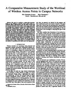
Figure 3: (a) Topology of the outdoor 20 mote setup for 0 dBm transmit power. Links shown have at least 99% PRR. This results in average degree of about 8. (b) CDF of RSS observed in this testbed. (c) Google Maps image of the parking lot environment where the testbed was deployed. a static 20 motes testbed deployed indoors in a quiet office environment. The 20 motes are placed in a random fashion on a 7.5 ft long, 6 ft wide tabletop (Figure 2(c)). Since this testbed is exercised the most, the motes are powered through their USB interface from power outlets for convenience. Transmit powers from the lower range are chosen for this setup according to the area of deployment. This enables multiple simultaneous transmissions without making the resulting network graph too sparse. The resulting network topology for the testbed when a transmit power of -32.5 dBm is used is shown in Figure 2(a). The average degree of the nodes in the network graph comes out to be about 9. The cumulative distribution function of received signal strength (RSS) observed at receivers of all 380 links for three different transmit powers is shown in Figure 2(b). These are the three power values that would be used later in our experiments in this testbed.Also the CDF of aggregate data is shown. This shows that the RSS is well distributed over a range. Outdoor testbed with 20 nodes: The final setup consists of 20 motes placed outdoors in an open parking lot. (See Figure 3(c)). This testbed was temporarily setup on a weekend when there were sufficient empty spaces. The nodes are placed in a grid like topology as shown in Figure 3(a) for convenience. These motes are powered through batteries since there is no easy way to power them through USB in an outdoor environment. While the previous tabletop testbed uses transmit powers from the lower end, this setup uses the highest possible transmit power, 0 dBm.4 The cumulative distribution function of received signal strength (RSS) values observed at receivers of all 380 links for this setup is shown in Figure 3(b). We end this section with a note on power. We have noticed that use of battery power reduces transmit range. This might mean that the transmit power set by the program is not the transmit power actually used, depending 4 The setup and choice of powers are somewhat related. For an interference study, we need a setup where there are enough concurrent transmissions possible on some links, as well as there are enough opportunities of interference on others, both individual and cumulative. Otherwise, there is a possibility of arriving at trivial conclusions. This can arise when the network is very sparse where many concurrent transmissions are possible with little interference, or when the network is very dense where hardly more than one transmission possible at a time.

on power sources. Thus, it will not be appropriate for the reader to compare range and related data across experimental testbeds, as we have used different power sources in different cases (USB/mains and battery). However, range and related parameters are profiled separately for the indoor and outdoor scenarios. So, these differences do not play any role in our results.

3.

BUILDING PHYSICAL INTERFERENCE MODEL

The physical interference model describes the success probability of a transmission (modeled in terms of packet reception rate or PRR) when one or more interferers are contributing to the interference at the receiver of the intended transmission. If S is the signal power received at the intended receiver from the sender, N is the noise power at the receiver and ΣI is the sum of the interference powers experienced at the receiver caused by the group of interferers (transmitting concurrently), the model predicts the relationship between the bit error rate (BER) and SINR, where S SINR = ΣI+N . This relationship depends on radio properties such as modulation. The packet error rate (PER) is directly related to BER and depends on coding. The packet reception rate (PRR), a quantity we will evaluate directly, is simply 1 − PER and thus again is directly related to SINR. Typically, the PRR vs. SINR curve makes a sharp transition from low to high PRR values with increasing SINR. The rising part of the function has been described as the transition region in [36]. Since scheduling applications need a ‘binary’ model, the curve is typically ‘thresholded’ and is described as a step function changing from 0 and 1 at a specific value of SINR, called the SINR threshold or capture threshold. This variant of the physical model is henceforth referred to as thresholded physical interference model. The original model will be called the graded physical interference model.

3.1

Modeling with Single Interferer

To build the physical model, one needs to find the PRR vs. SINR relation. We do this empirically by simply taking many measurement samples of S, I and N for the three node setup (Section 2.4) – sender, receiver and interferer, thus diS . The samples vary in the rectly computing SINR as I+N values of S and I. This variation is obtained by changing the distances between transmitter-receiver and interferer-

receiver pairs. The transmitter receiver distance is varied from 1 foot to 64 feet5 in discrete steps. For each such transmitter-receiver distance, the interferer-receiver distance is also varied from 1 foot to 64 feet. The following measurements are performed in three successive steps for each transmitter-receiver and interfererreceiver distance pair. Each experiment in each step is preceded by the base station sending command message(s) and followed by the base station sending poll messages to collect the data. All packet transmissions in the testbed are done with 128 byte packets. 1. Noise estimation: Noise is measured by sampling the RSS register in the CC2420 radio when there is no other transmission. The receiver samples its RSS register every 20 ms for a period of 6 seconds. Using the valid values thus obtained6 the average noise at the receiver in the network is computed. 2. Pairwise RSS measurement: Transmitter and interferer take turn to send 1000 packets in succession to the receiver. Each packet transmission time is approximately 4 ms. The receiver samples the RSS register every 3 ms to obtain RSS on its link with the corresponding sender. (More frequent sampling did not change the measured RSS.) It is possible that some of these samples may have been taken when the sender is not transmitting. Such samples are filtered out from the dataset by comparing it with the noise estimate obtained in step 1. The average of RSS value from transmitter is taken as S, while the RSS from interferer is taken as I for calculating the SINR. This entire step is repeated for 8 different transmit powers covering the entire transmit power range of CC2420 radio from -32.5 dBm to 0 dBm. In all, this results in 64 experiments. 3. Concurrent transmission: In each experiment, the transmitter and the interferer ‘concurrently’ transmit 1000 packets each. The receiver records the number of packets it received correctly from the transmitter. This defines the packet reception rate (PRR) for the transmitterreceiver link in the presence of the interferer. This step is also repeated for 8 different transmit powers covering the entire transmit power range of CC2420 radio from -32.5 dBm to 0 dBm to exactly correspond to the step 2 above. The above three steps are done in succession so that noise and RSS measurements (in steps 1 and 2) are as fresh as possible when PRR is measured in step 3. This is to avoid any form of noise/RSS fluctuations over time. In the measurement time period we did not observe any statistically significant fluctuations. For example, when steps 1 and 2 are repeated we obtained samples statistically similar as before. For each PRR obtained in step 3 above, the SINR is calculated using measurements from step 1 and 2. A scatterplot showing the results of this experiments is shown in Figure 4. The results show that for SINR greater than about 5 dB, 5 The TelosB datasheet [1] documents that its indoor RF range upto 64 feet. 6 Not all read attempts for the register produce valid values [31].

1 0.9

Measured Fitted curve

0.8 0.7

PRR

0.6 0.5 0.4 0.3 0.2 0.1 0 -10

-8

-6

-4

-2 0 2 SINR (dB)

4

6

8

10

Figure 4: PRR vs. SINR relation for single interferer measurements on a 3 node setup. The fitted curve on the aggregated data (bold,red) is shown for reference. PRR is almost 100%. As mentioned before, there is a transition region [36] between (−3) to 5 dB where packets are received with a probability less than 1. This region is somewhat noisy and predictability is poor (also observed in [36] albeit for a different radio). The PRR trails down to 0 below (−3) dB. We also show a fitted curve using a linear interpolation of average values in buckets of 1 dB each. This fitted curve provides the PRR vs. SINR model that will used in our later analysis. This model can also be used directly by a scheduling algorithm.

3.2

Validation with Multiple Interferers

While in theory the physical model is dependent only on the received powers and not on the number of interferers, previous work has made an observation in the contrary, albeit for an older generation radio (CC1000) [29]. Much was attributed to hardware imperfections and measurement noise. Since we undertake a measurement-based paradigm, it is of interest to validate the above empirically derived model in presence of multiple interferers. In the next subsection, we will also extend this validation for multiple channels and multiple transmit powers. These validations are key to assumption that only received powers drive the model and not any other parameter. We develop a systematic methodology for validation with multiple interferers. Let us denote by RSSrp (s) the received signal strength at node r when a node s transmits with transmit power p; and by Nr the ambient noise at r. Assume that a set of nodes, Φ, is active simultaneously transmiting at power p. Then, we also denote the PRR at r from a node i ∈ Φ as P RRrp (i, Φ). In this case, the SINR at r for node i is given by RSSrp (i) X SIN Rrp (i, Φ) = (1) Nr + RSSrp (j) ∀j∈Φ,j6=i

SIN Rrp (i, Φ) above can be computed from individual pairwise RSS measurements done separately. P RRrp (i, Φ) can be directly measured by making the nodes in Φ transmit together at power p and by measuring PRR at node r for packets transmitted by i. This provides a data point for the PRR vs. SINR relation. In fact, just one single experiment with the nodes in Φ transmitting together can provide PRR at any node r ∈ / Φ for each sender i ∈ Φ. Such experiments can be repeated for different Φ and p in different settings, providing many data points for the PRR vs. SINR relation. Similar measurements as in Section 3.1 are performed in three successive steps on the 20-node indoor testbed to this

end. Only one transmit power is used (−32.5 dBm). One other important difference here is that there are more than one interferer and thus more than two concurrent transmitters, i.e., Φ > 2. This makes step 3 only slightly more elaborate. Here, a set of nodes Φ ‘concurrently’ transmit 1000 packets each. All nodes r ∈ / Φ act as receivers. Each receiver records the number of packets it received correctly from each transmitter. This defines the packet reception rate (PRR) for different links in presence of a set of interfering transmissions. The set Φ was chosen randomly out of the 20 nodes in the network. The size of set Φ was varied from 3 to 6. 100 such random sets are used for each chosen value of |Φ|. At the end of the measurement process, we have 100 × |Φ| × (20 − |Φ|) data points for the PRR vs. SINR relation for each |Φ|. We show these as scatterplots in Figure 5 categorizing into different values for |Φ|. For brevity, only 4, 5 and 6 transmitter cases are presented, which means 3, 4 and 5 interferers, respectively. This categorization is specifically intended to demonstrate that the relationship is independent of the number of interferers and interference does work in an additive fashion as the theory predicts (at least upto the extent of 5 interferers that we could study). The fitted curve developed in the previous subsection is shown as well for comparison. Note the excellent fit. The coefficient of determination (R2 ) values for these experiments with respect to the fitted curve is always over 0.90. In a separate work [16], we conducted more extensive experiments to verify the additive nature of interference. The results reported there revealed excellent agreement between measured aggregated interference and sum of the individual RSS’s from the interferers with R2 = 0.99. It shows that the observations in [29] is quite likely due to imperfections and high degree of measurement noises in older generation hardware.

3.3

Validation with Multiple Channels and Transmit Powers

So far, we have used only one channel (channel fA ) and the same transmit power (-32.5 dBm) in our multiple interferer modeling experiments. Since often scheduling protocols use multiple channels (see, e.g., [3]) and different transmit powers (see, e.g., [5]) to exploit diversity, we want to also validate whether the PRR vs. SINR relationship depends upon transmit power or transmission channel. While an exhaustive evaluation is combinatorially explosive, we have carried out a large number of experiments to validate that the empirical PRR vs. SINR relationship obtained in Figure 5 does hold for various power levels and channels. For lack of space we report a subset of the results in Figure 6. The same methodology is followed as before. Step 2 is repeated with senders transmitting at three different transmit power levels and on three channels (See Section 2). Homogenous transmit powers have been chosen to reduce the number of experiments. Each experiment is repeated so that the receivers can measure noise and RSS in each channel. In step 3, the channels are selected randomly for randomly chosen set of transmitting nodes, Φ. A subset of results is shown in Figure 6 shown against the same fitted curve. Note that, generally speaking, the SINR vs PRR relation remains fairly independent of different transmit powers and use of multiple overlapping channels. We again have an R2 value of at least 0.90 for these results.

3.4

Discussions

While one could like a better overall confidence than 0.90, we attribute the remaining variations to hardware differences between individual motes and measurement errors. Given our experience vis-a-vis prior work [29], we feel that low-power radios have matured enough that a purely measurement-based SINR profiling independent of any other parameter is possible and is usable in scheduling studies. We have also investigated whether the analytical BER vs. SNR curves can be directly used instead of profiling the PRR vs. SINR relation via measurements. Such analytical curves can be derived from the knowledge of modulation/coding and the noise processes. See [12] for the analytical BER vs SNR curves for 802.15.4. We found that this curve is about 2 dB shifted towards the left from the fitted curve we have derived here. Much can be attributed to this difference – from measurement errors in the low-cost radio to the fact that spectral characteristics of interference is different than AWGN noise assumed in the analytical curve. Calibrating the analytical model with measurements would be interesting, but is of little value in the work we are pursuing here.

4.

PAIRWISE INTERFERENCE MODELS

One goal of our work is to experimentally compare interference models. Our comparison points will be various pairwise interference models that are commonly used in literature. They consider interference within only pairs of links as opposed to sets of links as in the physical interference model. The advantage of pairwise models is that the interference can be represented in terms of a conflict graph [13], which makes modeling and analysis straightforward. For example, for scheduling one simply needs to find an independent set of nodes in the conflict graph. In this section, we present the pairwise models and the empirical techniques used to instantiate the models. Before we describe the models, let us define some notations. Assume that the network graph is denoted by G(V, E). A communication link between two nodes u, v ∈ V (u is the sender and v is the receiver) is denoted by l(u, v) ∈ E. Assume that the physical distance between the two nodes is d(u, v). In the following, we enumerate the conditions under which each model predicts that a link l(x, y) interferes with another link l(u, v). These models consider this interference in a binary sense — PRR on l(u, v) will be 0 if l(x, y) interferes, else the PRR will be 1. This is make it amenable to conflict graph representation.

4.1

Description of Models

Hop-based model: Hop-based interference model [28] states that link l(x, y) interferes with link l(u, v), if node x is within k hops of v in the graph G. k is usually 1 or 2. Many scheduling works [27] have used this model to simplify the interference assumptions. Range-based model: The range based model uses two range or distance parameters, namely, transmission range (dT ) and interference range (dI ). It assumes that for any link l(u, v) ∈ E, d(u, v) ≤ dT . It also states that l(x, y) interferes with l(u, v), if d(x, v) ≤ dI . Many modeling and protocol studies [3] in wireless networks use such a model (often referred to as disk model). Range-based model is believed to be more accurate than the hop-based model, but it does not take into account the capture effect – if the sender

1

1

Measured Fitted curve

0.9

1

Measured Fitted curve

0.9

0.8

0.8

0.7

0.7

0.7

0.6

0.6

0.6

0.5

PRR

0.8

PRR

PRR

0.9

0.5

0.5

0.4

0.4

0.4

0.3

0.3

0.3

0.2

0.2

0.2

0.1

0.1

0 -10

-8

-6

-4

-2 0 2 SINR (dB)

4

6

8

0 -10

10

(a) 4 transmitters (3 interferer).

Measured Fitted curve

0.1 -8

-6

-4

-2 0 2 SINR (dB)

4

6

8

0 -10

10

(b) 5 transmitters (4 interferers).

-8

-6

-4

-2 0 2 SINR (dB)

4

6

8

10

(c) 6 transmitters (5 interferers).

Figure 5: PRR vs. SINR for different number of interferers. The fitted curve on (bold, red) is shown for reference. 1

1

Measured Fitted curve

0.9

1

Measured Fitted curve

0.9

0.8

0.8

0.7

0.7

0.7

0.6

0.6

0.6

0.5

PRR

0.8

PRR

PRR

0.9

0.5

0.5

0.4

0.4

0.4

0.3

0.3

0.3

0.2

0.2

0.2

0.1

0.1

0 -10

-8

-6

-4

-2

0

2

4

6

8

10

0 -10

0.1 -8

-6

-4

SINR (dB)

(a) single channel, power -25 dBm

Measured Fitted curve

-2

0

2

4

6

8

10

0 -10

-8

-6

-4

SINR (dB)

-2

0

2

4

6

8

10

SINR (dB)

(b) single channel, power -21 dBm

(c) multi channel, power -32.5 dBm

Figure 6: PRR vs. SINR results for 3 transmitters with different transmit powers and channels. Single channel experiment results with transmit powers of -25 dBm and -21 dBm are shown in (a) and (b) while multichannel experiment result with transmit power of -31.5 dBm is shown in (c). The fitted curve (bold, red) is shown for reference. and receiver are close enough, the packet can be successfully received even when there is an interferer present close by. Protocol model: The protocol model was first introduced in [11]. This model also assumes a concept of transmission range as before, i.e., for any link l(u, v) ∈ E, d(u, v) ≤ dT . The model also states that link l(x, y) will interfere with l(u, v) if d(x, v) ≤ (1 + ∆)d(u, v), where ∆ ≥ 0. This model improves on the range-based model by making interference dependent on the ratio of the distances between sender-receiver and interferer-receiver and thus tries to address the capture effect. ∆ is assumed to be independent of the distance d(x, v) and d(u, v). Link quality-based model: Models using any concept of distance or SINR require pairwise distance or signal strength measurements. This may not be feasible always. To address this we introduce a new model that defines interference based on link quality as measured by PRR in absence of interference from another link. In this model, link l(x, y) will interfere with l(u, v) if link l(x, v) has a PRR more than a given threshold (interference threshold ).7 It is also assumed that the link l(u, v) already has a strong quality, characterized by a high PRR (PRR larger than an given threshold called transmission threshold ). Note that transmission threshold must be larger than interference threshold. 7 Note that link l(x, v) may not exist in the network graph G. So consider it hypothetical.

4.2

Instantiating Models

Just like the physical model in Section 3 the above pairwise models must be instantiated. This means that various model parameters need to be determined. But unlike the physical model, for which we separately verified the additive nature of interference, the classical definitions of pairwise models are taken as the ground truth (as described in Section 4.1) and we just instantiate them through measurements. In our work, transmission threshold is set at 99%. All links with PRR equal or more than 99% are considered links in the network graph G. Using this definition of link, we say that an interferer interferes with a link if the concurrent transmission from the interferer and the transmitter causes the receiver to receive less than 99% of packets from the transmitter. Using this definition of interference, we perform experiments to instantiate various models. We follow a similar methodology with the three node setup as in Section 3.1 (single interferer modeling). To instantiate the range-based model, the following technique is used. The distance between the transmitter and the receiver is slowly increased from a very small value. The transmit power is kept constant. The PRR of link from the transmitter to the receiver drops below 99% at some distance. This distance is the transmission range, or dT . To measure the interference range, dI , we first keep both the transmitter and the interferer at distance dT from the receiver. Then the interferer is slowly moved further away from the receiver. For each such distance, PRR is measured

Model Hop-based Range-based Protocol Link quality-based Physical (thresholded) interference Physical interference (graded)

Parameters for indoor scenario (Transmit power = −32.5 dBm) k =1 (1 hop) dI = 45 inch ∆ = 0.36 interference threshold = 0.0 PRR vs. SINR model (Sec. 3) SINR threshold = 5 dB PRR vs. SINR model (Sec. 3)

Parameters for outdoor scenario (Transmit power = 0 dBm) k =1 (1 hop) dI = 255 inch ∆ = 0.67 interference threshold = 0.0 PRR vs. SINR model (Sec. 3) SINR threshold = 5 dB PRR vs. SINR model (Sec. 3)

Table 1: Summary of model parameters used in experiments. at the receiver, when both transmitter and interferer are active concurrently. The PRR usually starts close to 0% and increases with increasing distance of the interferer. The distance at which PRR on transmitter-receiver link crosses 99% is taken as the interference range, dI . For the protocol model, we use ∆ such that dI = (1 + ∆)dT . Values of dI and dT are obtained from the above experiments. Since, ∆ should not depend on the distances between transmitter-receiver or interferer-receiver, any pair of distances which cause interference should suffice. Thus, using dI and dT is sufficient. The link quality-based model is instantiated in a similar manner by using an interference threshold such that the PRR on the transmitter-receiver link drops below 99%. This directly corresponds to the PRR on the interferer-receiver link when interferer is at distance dI from receiver and the transmitter is at distance dT from the receiver. For hopbased model, k=1 (one hop) as well as k=2 (two hop) models are evaluated. It was found that one-hop model gives better accuracy and is thus considered henceforth. The above instantiation experiments are performed both for the indoor and outdoor 20 nodes testbeds separately using transmit power of −32.5 dBm and 0 dBm respectively. The resulting parameters are listed in Table 1. For completeness the physical interference models are also included here.

5.

COMPARING INTERFERENCE MODELS

Our goal here is to compare various pairwise interference models with the SINR-based physical model for TDMA transmission scheduling. Since scheduling essentially determines ‘feasible’ transmission sets (links) in each slot subject to an interference model, a model’s responsibility is to describe which sets of links are feasible together and which are not. As evaluating all sets of links is intractable (there are exponentially many such sets), the best way to compare the interference models is to do a sampling study by comparing modeling accuracy in predicting the feasibility of a randomly chosen set of links. The measure of modeling accuracy is simply the difference between the measured throughput for the chosen set of links and the predicted throughput per the given model. We conducted the experiments in two different setups – our 20 node indoor testbed and the 20 node outdoor testbed, as described in Section 2.4. We used -32.5 dBm transmit power in the indoor testbed and 0 dBm in the outdoor testbed. All links with PRR (in absence of interference) equal or more than 99% are considered links in the network graph G. It is possible that if the transmission threshold is

chosen to be very different certain models may behave more conservatively or aggressively leading to somewhat different conclusions than we will make here. For brevity, we stick to a single choice of transmission threshold in this paper that signifies quite strong network links.

5.1

Use of Random Matchings

For the sampling study as mentioned before, it is possible to do some optimizations. Any scheduling algorithm must avoid the so-called primary interference, i.e., interference between links with a common endpoint in the network graph. Thus, the algorithm must choose a matching 8 on the network graph as we are only considering unicast transmissions. Thus, instead of using random subset of links, we can use random matchings. There is no point in evaluating nonmatchings as they will never be scheduled by any algorithm. Interestingly, use of matchings does not necessarily reduce the complexity of the problem as there can be exponentially many matchings. Thus, we still need to do random sampling. Choosing random matchings is intractable as well. Thus, we resort to a heuristic to pick random matchings. The heuristic is described in the Appendix. About 13,000 random matchings are used for the indoor experiments and about 3,000 for the outdoor, providing significant data sets. Such large data set also makes the study relatively independent of the topology used. This is because we could independently verify that the data set included many instances of links well distributed over the relevant range of SINR values. For each randomly selected matching the actual throughput (normalized) of each link is evaluated when all links in the matching are transmitting concurrently in the testbed. The normalized throughput is simply the number of packets received on each link divided by the number of packets transmitted on this link. For each matching, 1000 concurrent transmissions are done over all links in the matching to calculate throughput.

5.2

Modeling Error

Each random set of matching is used as input to a predictor that evaluates the link throughput predicted by each interference model discussed in Sections 3 and 4. Note that all links in a given matching may not be deemed feasible by a given interference model. Thus, for the binary models, the throughputs of all conflicting links in a matching are assumed to be 0 and those of the non-conflicting links are assumed to be 1. For the physical model, the throughputs are simply the PRRs as determined by the PRR vs. SINR 8 A matching is a set of links such that no two links have a common end point.

100

90

90

80

80

70

70 Percentage of links

Percentage of links

100

60 50 40

60 50 40 30

30 Physical (Graded) Physical (Thresholded) One hop Link quality Range Protocol

20 10

10 0

0 -1

-0.8

-0.6

-0.4

-0.2

0

0.2

0.4

0.6

Physical (Graded) Physical (Thresholded) One hop Link quality Range Protocol

20

0.8

1

0

0.1

0.2

0.3

0.4

Errors

0.5

0.6

0.7

0.8

0.9

1

Errors

(a) Actual error.

(b) Absolute error.

100

100

90

90

80

80

70

70 Percentage of links

Percentage of links

Figure 7: Indoor testbed (-32.5 dBm transmit power): CDF of modeling errors (per Equation 2) for different interference models. (Absolute error is simply the absolute value of the actual error.)

60 50 40 30

60 50 40 30

Physical (Graded) Physical (Thresholded) One hop Link quality Range Protocol

20 10

Physical (Graded) Physical (Thresholded) One hop Link quality Range Protocol

20 10

0

0 0

0.1

0.2

0.3

0.4

0.5

0.6

0.7

0.8

0.9

1

Errors

0

0.1

0.2

0.3

0.4

0.5

0.6

0.7

0.8

0.9

1

Errors

(a) Absolute error in transition region.

(b) Absolute error in non-transition region.

Figure 8: Indoor testbed (-32.5 dBm transmit power): CDF of absolute modeling errors (per Equation 2) for different interference models, with data split into transition and non-transition regions. relation. The modeling error is evaluated in the following fashion. Given a matching Mi consisting of |Mi | links we denote the measured throughput for j-th link in this matching as Γji (measured) and the predicted throughput by model k as Γji (model(k)). Then the modeling error for the interference model k with respect to the j-th link in the matching Mi is given by errorij (model(k)) = Γji (measured) − Γji (model(k)).

5.3

(2)

Experimental Results

Experiments are performed in the two 20-node testbeds. For the indoor testbed the lowest transmit power (-32.5 dBm) and for the outdoor testbed the highest transmit power (0 dBm) are used. The cumulative distribution function (CDF) of the modeling errors (Equation 2) is plotted to compare various interference models. Figure 7 and Figure 9 show the CDF plots for indoor and outdoor testbeds respectively. Note that the very smooth nature of the indoor results is due to a very large dataset (13,000 matchings).

From the CDF results, we can see that overall the graded physical interference model is the most accurate. The 90percentile error is about 0.25 for indoor and about 0.2 for outdoor experiments. The 80-percentile error is down to 0.07 and 0.12, respectively. Also, note that while the accuracy is good, it is not excellent. We will come back to this question momentarily. The thresholded physical model is a close second to the graded model, with 80-percentile error close to zero for indoor and 0.15 for outdoor experiments. But the 90-percentile error for the thresholded model is very high, close to 0.9 for indoor and 0.6 for outdoor. This high error is due to the fact the thresholded physical model is quite accurate for links outside the transition region, but links in the transition region are predicted to have zero throughput. The percentage of links which lie in transition region for our experiments is approximately 20%. Thus thresholded model gives large error for 20% of cases. The pairwise models have higher error. The best one among them roughly trails the physical model by 12-18 percentile points for the same error target. They also exhibit

100

80

80

Percentage of links

Percentage of links

100

60

40

Physical (Graded) Physical (Thresholded) One hop Link quality Range Protocol

20

60

40

Physical (Graded) Physical (Thresholded) One hop Link quality Range Protocol

20

0

0 -1

-0.5

0

0.5

1

0

0.2

0.4

Error

0.6

0.8

1

Error

(a) Actual error.

(b) Absolute error.

100

100

80

80

Percentage of links

Percentage of links

Figure 9: Outdoor testbed (0 dBm transmit power): CDF of modeling errors (per Equation 2) for different interference models. (Absolute error is simply the absolute value of the actual error.)

60

40

Physical (Graded) Physical (Thresholded) One hop Link quality Range Protocol

20

60

40

Physical (Graded) Physical (Thresholded) One hop Link quality Range Protocol

20

0

0 0

0.2

0.4

0.6

0.8

1

Error

(a) Absolute error in transition region.

0

0.2

0.4

0.6

0.8

1

Error

(b) Absolute error in non-transition region.

Figure 10: Outdoor testbed (0 dBm transmit power): CDF of absolute modeling errors (per Equation 2) for different interference models, with data split into transition and non-transition regions. some interesting characteristics. Note the nature of the absolute error plots (Figure 7(b) and 9(b)) – first a sharp rise near 0, then relatively flat and then again a sharp rise near 1. This denotes a bimodal error distribution – most errors are either very low or very high. The reason for this is the binary nature of these models. Note also some of these models have significant bias, they tend to either under-estimation or over-estimation (see Figures 7(a) and 9(a)). Sometimes this bias is not even consistent. This happens for the range-based model that over-estimates in the indoor scenario and underestimates in the outdoor scenario. Much of these problems is related to the fact that these models depend on estimation of a single model parameter. Among these models, the hop based and the protocol model perform relatively better, but this is again scenario-specific. Now, let us get back to modeling accuracy question for our best model – the graded physical model. It was observed before, albeit with an older mote/radio platform [36], that the links in the transition region are hard to estimate accurately. This is because a slight measurement error makes a signif-

icant difference in the estimate. To investigate this issue further in our platform, we split out the results presented in Figures 7(b) and 9(b) into two parts, for the transition and non-transition regions. Recall that from our model instantiation experience in Section 3, we found that the transition region for CC24020 radio is −3 to 5 dB. The new plots are shown in Figures 8 and 10. Note the poorer accuracy of all models in the transition region relative to the non-transition region. But the graded physical interference model still performs better than all other models. The thresholded physical model does much worse than the graded physical model in the transition region. It performs as bad as the other pairwise models. It is interesting to note that both graded and thresholded physical models are very accurate for the non-transition region case, 90-percentile error is about 1% for the indoor setup and 80-percentile error is about 1% for the outdoor scenario. We summarize our general findings below: 1. Generally speaking, the graded physical interference model outperforms any other. However, the overall

accuracy is not perfect, particularly in outdoors.

3. The best performing pairwise model is about 12-18 percentile points poorer than the physical model depending on the environment and error target. 4. If a pairwise model must be used, either protocol or hop-based approach should be preferred. Hop-based model worked well in our indoor experiments and the protocol model for outdoor experiments. 5. The range-based model, while widely used in literature, performs quite poorly in both testbeds. This is even with relationship to a much simpler hop-based model.

6.

EVALUATING SCHEDULING PERFORMANCE

The previous section evaluated the accuracy of various interference models in predicting the feasibility of a randomly chosen set of links. While these evaluations are very comprehensive, they only evaluate modeling accuracy, but do not directly model real performances when used in a scheduling algorithm. This is because a scheduling algorithm considers only specific subsets of links for feasibility. This is entirely algorithm dependent. To gain some insight here, we now study the performance of various interference models for making actual scheduling decisions. We limit our work only to the indoor testbed using transmit power −32.5dBm. Our work here is split into two parts. First, we study all models using a greedy scheduling algorithm – similar to the one used in literature [6, 28, 34] – for scheduling all links in the network. The graded physical model, however, cannot be considered here, as no scheduling algorithm exists in current literature to account for the probabilistic (non-binary) behavior in this model. So, in the second part, we separately consider the graded model and evaluate its performance for a simplified scheduling problem (one-shot scheduling [8]).

6.1

Scheduling All Links Using Greedy Algorithm

For a fair comparison, we use the same greedy scheduling algorithm for all models. It is simple to implement and performance bounds are known for specific models [4, 6, 28]. The link demand vector is an input to the algorithm. The demand for a link is simply the number of packets to be scheduled on the link. The schedule is a sequence of slots with a feasible set of links to be scheduled in each slot. In our implementation, each slot is equivalent to one packet (128 bytes) transmission and processing time in the mote (12.5ms). The greedy algorithm works as follows. Input: Network graph G = (V, E), demand vector on the links f = (f1 , . . . , f|E| ) and interference model. The interference model specifies which set of links are ‘feasible’ together. Output: Schedule S = {S1 , S2 , . . . , Sτ }, where Sk is a feasible set of links scheduled in the same slot. τ is the schedule length. Algorithm:

2.5 Packets/slot

2. If a binary interference model is to be used (all existing scheduling algorithms rely on such models), thresholded physical model is still the best overall, but this is worse that the graded model.

3

2 1.5 1 0.5 0 Demand Vector 1 Physical (Thresholded)

Demand Vector 2 Link Quality

Demand Vector 3 Range

Protocol

Demand Vector 4 One hop

Figure 11: Measured aggregate throughput for various interference models for four different link demand vectors (indoor testbed, -32.5 dBm transmit power). 1. Order and rename links such that f1 ≥ f2 ≥ f3 . . . ≥ f|E| . 2. Set i = 1, S = φ, τ = 0. (Initial schedule is empty.) 3. Schedule link i in the very first available slot where it can be scheduled interference-free according to the given interference model. If no such slot of feasible, increment τ and schedule the link in the last slot. (Incrementing τ is equivalent to creating a new empty slot at the end of the current schedule.) 4. Repeat step 3 above fi times. 5. Increment i. Go back to step 3 until i > |E|. The physical (thresholded), link quality-based, Range-based, protocol and 1-hop models are considered. As mentioned before, the graded physical model is not considered as the greedy algorithm handles feasibility in a binary sense (either feasible or not). This model will be considered separately in the next subsection. The models are compared in the following fashion. Different models generate different schedules for a given demand vector. Four different demand vectors are considered for experiments. The links are split into two equal sets randomly. One set has one packet each. The other set has i packets each for vector i. The schedules generated by each model are evaluated using direct TDMA scheduling experiments on the testbed. Due to modeling inaccuracy some slots may have links scheduled that are infeasible in the experiments. This leads to packet losses. The lost packets are retransmitted. To do this, fresh schedules are computed with only packets lost in the previous attempt constituting link demands. All schedule computation is done by the ‘base station’ which also has access to all packet loss information (see section 2). This procedure is repeated until all packets are successfully transmitted.9 The above constitutes one 9 Note that this strategy may get ‘stuck,’ where links scheduled in one slot are all infeasible in reality, and the same links are scheduled in one slot again during retransmissions. This will lead to repeated losses as the same scheduling pattern will continue. This could be addressed (but not perfectly resolved) via randomizing the order of the links considered in the algorithm. We did not, however, see this behavior in our experiments. Note that this is a fundamental problem for

trial. Trials are repeated 1000 times for each demand vector and the performance is averaged to determine the measured aggregate throughput in packets/slot. The results are presented in Figure 11. As expected, physical model has the best throughput, 1-hop model a close second, losing about 5%–20% of throughput. The range-based model generally performs the worst, losing more than 40% of throughput in all cases. The results here are in general agreement with the observations in the previous section (see Figure 7) except for the link quality model. Relative performance of this model is better in scheduling than what we saw before. This is likely due to significant conservative estimates (note large positive errors in this model in Figure 7) in this model that works favorably here. This is because the given demand vectors have packets on all links.

6.2

Graded vs. Thresholded Physical Model: One Shot Scheduling

We did not consider the graded physical model above as the greedy scheduling can only use a binary model (links are either feasible or not). However, the graded model has proved to be the most accurate in our evaluations in Section 5. So, it is also instructive to investigate its potential for scheduling. The thresholded model does perform excellently outside the transition region, but its performance is quite poor in the transition region. The graded model, while not excellent in the transition region either, is still much better than its thresholded counterpart. For example, in the indoor case, the 70-percentile error in the graded model is about 20%, while in the thresholded model it is close to 90% (see Figure 8a). A natural question arises: Can this improved accuracy for the transition region be gainfully used in scheduling? Another way to argue this would be to say that the thresholded model is unduly conservative. It only allows transmissions with very high (close to 1) probability of success. Can we gain extra capacity by allowing transmissions with less than perfect success probability? Note that extra capacity could be substantial if there are many links in the transition region.10 To address this question we need to develop new scheduling algorithms that can treat links as non-binary. A comprehensive treatment of this topic is beyond the scope of this paper, where we want to focus on measurements only. However, to make our observations stronger, we study here a simplified scheduling problem called “One Shot Scheduling” [8] and experiment with scheduling algorithms both for graded and thresholded physical interference models. The one shot scheduling problem picks a subset S of links to be scheduled from a given set L such that the aggregate throughput is maximized. We redefine throughput as ‘expected throughput’ as we are dealing with probabilistic transmission success. The one shot scheduling problem for the thresholded physical model is intractable [8]. But, for small size of L, it is computationally feasible to exhaustively look for the optimal subset Sopt to be scheduled. Any set of schedulable links has to be a matching. Thus, we can pre-select L as a matching. With a 20 node network |L| is upper-bounded by 10. Thus, exhaustive search is feasible using an inaccurate interference model, and does not have a perfect solution. 10 We are sometimes using the expression “links in transition region” to mean links with SINR in the transition region.

to obtain optimal schedules for both models. One needs to evaluate only 1024 possibilities. The experiments are done on the indoor testbed as follows. First, we obtain the connectivity graph of the network. Since we are comparing only physical models, here we define network links as those with SNR greater than the the SINR threshold (5 dB). For each experiment, we pick a random matching L from the connectivity graph such that the |L| is equal or close to 10. For each model, we estimate the throughput of each subset S of L and then choose the optimal subset Sopt which provides the maximum aggregate throughput. Note that the Sopt for the graded model can be different than Sopt for the thresholded model. Thus, for each experiment, we schedule both these subsets one by one in the testbed to find their respective throughputs (using a process similar to used in Section 5). The receiver for each link records the respective PRR and the base station collects this information at the end of the step and determines the aggregate throughput. We perform 50 such experiments with different random choice of L each time and each experiment is repeated 5 times to obtain an average throughput for each model as well as confidence intervals. The results are shown in Figure 12. Throughput is expressed in terms of average number of packets successfully transmitted per slot. This is the Y-axis. The individual experiments (i.e., different choices of L) are shown on the X-axis, sorted in the order of increasing throughput for the graded model for visual clarity. For each experiment, the throughput for thresholded model is drawn as a bar graph on the left while the throughput for graded model is drawn on the right. 95% confidence intervals are shown using error bars. They are usually very small, particularly for the thresholded model. The model predictions are also shown. It is easy to see that in 90% of the experiments, graded model gives higher throughput. Overall, the graded model got 3.14 packets/slot successfully transmitted per experiment while thresholded model got 2.45 packets/slot. This is an improvement of about 28%. However, the modeling error (difference between predicted and measured throughput) is significant for the graded model in about 30% of the cases, while this is true only for 10% of the cases for the thresholded model. This is expected as the graded model schedules links in the transition region that has relatively poor predictability. However, we do see that the thresholded model is not perfect either. This simple one shot scheduling experiment shows the power of using graded physical interference model instead of using the more conventional thresholded model for use in scheduling. We expect that the general observations here applies for other types of wireless networks also, and not just with low-power radio links.

7.

RELATED WORK

A recent paper by Brar et al. [6] can be considered complimentary to our work. Here, the authors investigate algorithms for physical model and show via simulations that physical interference modeling leads to more efficient schedules relative to the protocol model. However, the simulations use very straightforward propagation and radio models. We also arrive at similar conclusions, albeit via a more elaborate experimentally based method, but in the context of low-power wireless links. Researchers have only begun to study effect of interfer-

Packets per slot

5 4.5 4 3.5 3 2.5 2 1.5 1 0.5 0 1

3

5

7

9

11

13

15

17

19

21

23

25

27

29

31

33

35

37

39

41

43

45

47

49

Experiment # Thresholded Measured

Graded Measured

Thresholded Predicted

Graded Predicted

Figure 12: Results of the One Shot Scheduling experiment comparing the thresholded vs. graded physical interference models (indoor testbed, -32.5 dBm transmit power). ence in wireless networks using experimental methods. The authors in [36] have studied the transition region and quantified its effects. The analysis in the paper is also supported by experimental validation using a motes testbed, though with a different (CC1000) radio. Many of our observations are also similar. Another work [29] by the same group has considered the effect of multiple interferers. They however concluded that the SINR threshold is dependent on number of interferers and the joint interference is not necessarily the sum of individual interference powers. They also observed slightly different behaviors dependent on received power ranges. As described in Section 3, our conclusions are somewhat different with the newer radio platforms, and we have derived a more classical model [24]. In a different work [30], the authors have concluded from measurements on MicaZ motes with CC2420 radios, that RSSI is a good estimate of link quality. This observation is also confirmed by the success of our SINR-based models. In another work [35], the authors investigated the accuracy of the range-based interference model by conducting experiments with Mica2 motes. They concluded that it is inaccurate and proposed a new protocol to detect run-time radio interference relation among nodes. Our results also point out the inaccuracies in range-based models. Experimental work has also considered 802.11-based systems to study interference behavior. The difference here is that the sender-side (carrier-sense) behavior in the MAC protocol must also be modeled. This phenomenon is absent in TDMA scheduling. Notable articles are as follows. Single and multiple interferer scenarios have been modeled in [25] and [14,23], respectively. The need for modeling ‘graded’ interference has been demonstrated in [22]. The need for modeling multiple interferers has been motivated in [7]. Techniques for generating interference maps have been developed in [21]. [15] has investigated the capture effect.

8.

CONCLUSIONS

There are several contributions in this work. First, we develop and validate a purely measurement-based method to instantiate SINR-based physical interference model. Second, we compare the accuracy of different interference models via extensive experimentation on two different motes testbeds – low power, indoors and high power, outdoors. The general

conclusion is that the physical interference model provides the best accuracy. But it is still far from being perfect (90percentile error about 20-25%). Many commonly used models such as hop-based, range-based and protocol model have poorer accuracy. In case a pairwise model must be used, our experience indicates that the range-based model should be avoided. This provided the worst performance across the board, while the experience with other models varied. Third, we observe that while the thresholded physical interference model is used in existing scheduling algorithms, it is overly conservative and does not utilize links in the so-called transition region. We have shown the potential of scheduling such links by directly using the graded physical model in a scheduling problem. We expect that this observation will generate new research in exploiting the graded nature of the physical model for better scheduling. As a part of our future work, we will strengthen the observations made here with more scenarios. Also, our general methodology is radio-independent. Thus, it will be interesting to carry out similar experiments on other commodity radio platforms. Use of CSMA as a MAC layer model is also an interesting direction. In this case, modeling link or path capacities for different upper layer uses (e.g., routing) for different interference models is a promising direction. Some work in this direction has already been done [14, 23], albeit using 802.11 protocol.

ACKNOWLEDGMENTS This work was partially supported by NSF grants CNS0751121, CNS-0721665, CNS-0721455, IIS-0713186, CNS0519734 and CNS-0423460; a grant from CONACYT, Mexico; and equipment support from the NY Center of Excellence in Wireless and Information Technology (CEWIT).

9.

REFERENCES

[1] “Moteiv,” http://www.moteiv.com. [2] “TinyOS community forum,” http://www.tinyos.net. [3] M. Alicherry, R. Bhatia, and L. E. Li, “Joint channel assignment and routing for throughput optimization in multi-radio wireless mesh networks,” in Proc. ACM MobiCom, 2005. [4] H. Balakrishnan, C. L. Barrett, V. S. A. Kumar, M. V. Marathe, and S. Thite, “The distance-2 matching

[5]

[6]

[7] [8] [9]

[10]

[11] [12]

[13]

[14]

[15]

[16]

[17]

[18] [19] [20]

[21] [22]

problem and its relationship to the MAC-layer capacity of ad hoc networks,” IEEE J. Selected Areas of Communication, pp. 1069–1079, 2004. S. Borbash and A. Ephremides, “Wireless link scheduling with power control and SINR constraints,” IEEE Trans. on Info. Theory, vol. 52, no. 11, pp. 5106–5111, 2006. G. Brar, D. M. Blough, and P. Santi, “Computationally efficient scheduling with the physical interference model for throughput improvement in wireless mesh networks,” in Proc. ACM MobiCom, 2006. S. Das, D. Koutsonikolas, Y. Hu, and D. Peroulis, “Characterizing multi-way interference in wireless mesh networks.” in Proc. ACM WiNTECH, 2005. O. Goussevskaia, Y. A. Oswald, and R. Wattenhofer, “Complexity in geometric SINR,” in Proc. ACM MobiHoc, 2007, pp. 100–109. B. Greenstein, A. Pesterev, C. Mar, E. Kohler, J. Judy, S. Farshchi, and D. Estrin, “Collecting high-rate data over low-rate sensor network radios,” Tech Report. Center for Embedded Network Sensing. Paper 17, 2007. http://repositories.cdlib.org/cens/techrep/17. J. Gronkvist and A. Hansson, “Comparison between graph-based and interference-based STDMA scheduling,” in Proc. ACM MobiHoc, 2001, pp. 255–258. P. Gupta and P. R. Kumar, “The capacity of wireless networks,” IEEE Transactions on Information Theory, vol. 46, no. 2, pp. 388–404, March 2000. IEEE Computer Society LAN/MAN Standards Committee, “802.15.4: Wireless medium access control (MAC) and physical layer (PHY) specifications for low-rate wireless personal area networks (LR-WPANS),” 2003. K. Jain, J. Padhye, V. Padmanabhan, and L. Qiu, “Impact of interference on multi-hop wireless network performance,” in Proc. ACM MobiCom, 2003, pp. 66–80. A. Kashyap, S. Ganguly, and S. R. Das, “A Measurement-Based Approach to Modeling Link Capacity in 802.11-based Wireless Networks,” in Proc. ACM MobiCom, 2007. J. Lee, W. Kim, S.-J. Lee, D. Jo, J. Ryu, T. Kwon, and Y. Choi, “An experimental study on the capture effect in 802.11a networks,” in Proc. ACM WiNTECH, 2007, pp. 19–26. R. Maheshwari, S. Jain, and S. R. Das, “On estimating joint interference for concurrent packet transmissions in low power wireless networks,” in Proc. ACM WiNTECH, Sept 2008. A. Mishra, V. Shrivastava, S. Banerjee, and W. Arbaugh, “Partially-overlapped channels not considered harmful,” in Proc. ACM SIGMTERICS, 2006. T. Moscibroda and R. Wattenhofer, “The complexity of connectivity in wireless networks,” in Proc. IEEE INFOCOM, 2006. Moteiv Corporation, Tmote Sky: Ultra low power IEEE 802.15.4 compliant wireless sensor module, San Fransisco, CA, November 2006. R. Nelson and L. Kleinrock, “Spatial-TDMA: A collison-free multihop channel access protocol,” IEEE Transactions on Communication, vol. 33, pp. 934–944, Sept. 1985. D. Niculescu, “Interference map for 802.11 networks,” in Proc. IMC. New York, NY, USA: ACM, 2007, pp. 339–350. J. Padhye, S. Agarwal, V. Padmanabhan, L. Qiu, A. Rao, and B. Zill, “Estimation of link interference in

[23] [24] [25]

[26]

[27] [28] [29]

[30] [31] [32]

[33] [34] [35] [36]

static multi-hop wireless networks,” in Proc. IMC, 2005. L. Qiu, Y. Zhang, F. Wang, M. K. Han, and R. Mahajan, “A general model of wireless interference,” in Proc. ACM MobiCom, 2007. T. Rappaport, Wireless Communication: Principles and Practice. Prentice-Hall, 2002. C. Reis, R. Mahajan, M. Rodrig, D. Wetherall, and J. Zahorjan, “Measurement-based models of delivery and interference in static wireless networks,” in Proc. ACM SIGCOMM, 2006. I. Rhee, A. Warrier, J. Min, and L. Xu, “DRAND: Distributed randomized TDMA scheduling for wireless ad hoc networks,” in Proc. ACM MobiHoc, 2006, pp. 190–201. I. Rhee, A. Warrier, M. Aia, and J. Min, “Z-mac: a hybrid mac for wireless sensor networks,” in Proc. ACM SenSys, 2005. G. Sharma, R. Mazumdar, and N. Shroff, “On the complexity of scheduling in wireless networks,” in Proc. ACM MobiCom, 2006. D. Son, B. Krishnamachari, and J. Heidemann, “Experimental study of concurrent transmission in wireless sensor networks,” in Proc. ACM SenSys , 2006, pp. 237–250. K. Srinivasan and P. Levis, “RSSI is Under-Appreciated,” in Proc. EmNetS, 2006. CC2420 Radio Datasheet, 1st ed., Texas Instruments, October 2005. W. Wang, Y. Wang, X.-Y. Li, W.-Z. Song, and O. Frieder, “Efficient interference-aware TDMA link scheduling for static wireless networks,” in Proc. ACM MobiCom, 2006, pp. 262–273. K. Whitehouse, A. Woo, F. Jiang, J. Polastre, and D. Culler, “Exploiting the capture effect for collision detection and recovery,” in Proc. IEEE EmNetS, 2005. X. Wu and R. Srikant, “Bounds on the capacity region of multi-hop wireless networks under distributed greedy scheduling,” in Proc. IEEE INFOCOM, 2006. G. Zhou, T. He, J. Stankovic, and T. Abdelzaher, “RID: Radio Interference Detection in Wireless Sensor Networks,” in Proc. IEEE INFOCOM, 2005. M. Zuniga and B. Krishnamachari, “Analyzing the transitional region in low power wireless links,” in Proc. IEEE SECON, 2004, pp. 517–526.

APPENDIX A. CHOOSING RANDOM MATCHING Assume, M is the matching to be picked randomly. We first choose |M |, the size of M . Ideally this should be chosen randomly based on the probability of choosing matchings of different sizes. Since this is a hard problem we use the probability of choosing a matching of size |M | ‘approximated’ |) to be C(|E|,|M , where C(n, k) is “n choose k.” Once the 2|E| size is picked randomly based on this probability, a random matching is computed by simply selecting random links in sequence and by putting them in a set so long as the set remains a matching. For some sizes, the sequence in which links are chosen may not provide a matching of the desired size. In such cases, this trial is discarded and a new random trial is used.