We use Soekris 4511 and 4826 boards [11] and Atheros 5213 chipset-based 802.11a/b/g mini-PCI cards manufactured by. Winstron connected to a 5 dBi ...
Physical Interference Modeling for Transmission Scheduling on Commodity WiFi Hardware Ritesh Maheshwari, Jing Cao, Samir R. Das Computer Science Department, Stony Brook University Stony Brook, New York 11794-4400, USA Abstract—The demand for capacity in WiFi networks is driving a new look at transmission scheduling based link layers, particularly in the context of mesh networks. One basic issue here is the use of accurate interference models to drive transmission scheduling algorithms. However, experimental work in this space has been limited. In this work, we use commodity WiFi hardware (specifically, 802.11a) for a comprehensive study on interference modeling for transmission scheduling on a mesh setup. We focus on the well-known physical interference model for its realism. We empirically build the physical interference model via a packet reception rate vs. SINR relationship using a measurement driven method. We propose use of the “graded” version of the model where feasibility of a link is probabilistic, as opposed to using the more traditional “thresholded” version, where feasibility is binary. We show experimentally that the graded model is significantly more accurate (80 percentile error 0.2 vs. 0.55 for thresholded model). However, the graded model has never been considered in algorithmic studies on transmission scheduling. Carrying on further, we develop transmission scheduling experiments using greedy scheduling algorithms for the evacuation model for both interference models. We also develop similar experiments for optimal scheduling performance for the simplified one-shot scheduling. The scheduling experiments demonstrate clearly superior performance for the graded model, often by a factor of 2.
I. I NTRODUCTION TDMA-based transmission scheduling can potentially extract the optimal capacity from a wireless network. On the other hand, CSMA-based MAC protocols, such as used in 802.11, are known to have poor performance in heavy traffic situations. Several measurement studies have documented this in real world scenarios [1], [2]. CSMA protocols are also not easily amenable to rigorous mathematical modeling for throughput and capacity [3]. The problem with 802.11 is expected to be worse in mesh networks, where high capacity backbone links are needed and multihop interference plays a significant role. This makes a case for developing robust TDMA-based transmission scheduling on 802.11 hardware using the existing 802.11 PHY layer. The reason this is attractive is that 802.11 platforms are now commodity, and firmware modifications to alter the standard MAC layer are possible to obtain new MAC functionalities [4], [5]. On the theoretical side, transmission scheduling algorithms and their performance bounds are wellinvestigated in literature [6]–[8]. Thus, a significant foundation is available to drive the above pursuit. However, practical questions remain. The algorithms are driven by an interference model. Consideration of unrealistic or inaccurate models hurts
performance in two obvious ways. Overly aggressive schedules may be infeasible in reality. Overly conservative schedules may not have enough concurrent transmissions even when they are actually possible. Neither is good for high throughput. Our goal in this work to understand this interference modeling aspect for transmission scheduling. We take a measurementdriven approach using commodity 802.11 hardware. It is important to note that developing a complete TDMA system on stock implementation of 802.11 PHY layer involves many aspects other than interference modeling and scheduling. Tightly synchronized time slots must be designed that are small enough. Traffic loads on the links must be estimated. Schedule must be computed and distributed with an appropriate centralized or distributed scheme. Overheads for all these must be minimized. Each of these independently are strong areas of research and consideration of all these would be beyond our scope. Our work here focuses on two basic aspects in this entire problem space: (i) interference modeling using measurements, (ii) studying actual scheduling performance on a 802.11 mesh testbed using known algorithmic approaches. There are several interference models that have been considered for transmission scheduling studies. They vary from oversimplified range-based models to fairly realistic SINRbased physical interference models [9]. Because of their realism, several recent studies have used physical models [6]–[8], [10]. The general goal here has been to develop algorithms to maximize throughputs, given specific traffic loads on the network links. However, all such works take a theoretical view of the problem, where they evaluate achievable capacity bounds or develop near-optimal algorithms. There is little knowledge in the community about practicality of such approaches. Our work is one of the first attempts to bridge this gap using a measurement-driven approach. We also address the modeling accuracy question and how it might impact scheduling performance. Physical models are based on SINR (signal to interference plus noise ratio). The relationship between bit error rate (BER) and SINR is exploited and it is assumed that if the SINR is sufficiently high, more than a given SINR threshold β, the BER is negligible and thus packet transmission is successful with very high probability. Lower SINR is not used for scheduling transmissions. We call such models “thresholded.” However, if we move away from the thresholded paradigm, lower SINRs can still be used for scheduling packet transmissions, albeit with non-negligible packet error rates.
Fraction of links
2
sniffer. This is because the sender’s signal is much stronger than any possible interferer. Note that the sniffer could be avoided if all actual packet transmissions in the air could be recorded on a transmitting 802.11 interface with accurate timestamps. However, commodity 802.11 interfaces and device drivers do not facilitate this.1
0.1 0.09 0.08 0.07 0.06 0.05 0.04 0.03 0.02 0.01 0 5 10 15 20 25 30 35 40 45 SINR (dB)
Fig. 1. Distribution of SINR for the links in the chosen activation sets in the testbed setup.
Depending on the application, this may require retransmissions from the link or upper layer. Thus, scheduling may directly use the actual BER vs SINR relation instead of thresholding it. We call this “graded” physical model. We show via real scheduling studies that graded models provide potential for higher throughputs, while only thresholded models have been considered in existing scheduling literature (e.g., [6]). The rest of the paper is organized as follows. In Section II, we describe the experimental setup of the 802.11a mesh network. In Section III, we describe how concurrent transmissions are acheieved for the purpose of this study. Section IV evaluates the accuracy of the two physical interference models. Section V investigates scheduling performance. Related work and conclusions are presented in Sections VI and VII, respectively. II. E XPERIMENTAL P LATFORM
AND
S ETUP
The mesh network testbed consists of 11 ‘network’ nodes. Each network node is monitored by a ‘sniffer’ node co-located with the network node, thus needing a total of 22 nodes in the testbed. The purpose of the sniffer will be explained momentarily. Each node is essentially a single-board computer (SBC), meant for embedded use, with an 802.11a/b/g interface. We use Soekris 4511 and 4826 boards [11] and Atheros 5213 chipset-based 802.11a/b/g mini-PCI cards manufactured by Winstron connected to a 5 dBi rubber-duck antenna. While the testbed uses two different types of boards, all 802.11 interfaces are identical. All experiments reported here are conducted in channel 44 of the 802.11a band using a single PHY layer rate 6 Mbps with transmit power of 11 dBm, and UDP packets with payload size 1470 bytes. These choices have been done with careful considerations to be discussed momentarily. The boards run pebble Linux with a mix of Linux 2.6.17 and 2.4.26 kernels with madwifi device driver version 0.9.4 for the 802.11 interface. The 802.11 interfaces in the network nodes are set up in ‘ad hoc’ mode and the sniffer nodes in ‘monitor’ mode. As mentioned before, each sniffer is co-located with the corresponding network node. The sniffer’s purpose is simply to record all packet transmissions from its corresponding network node. The sniffer does this by simply running a packet capture tool like tcpdump. The radiotap header supportis used so that RF level information (e.g., received signal strength (RSS) and noise powers) as well as accurate timestamps can be collected. More on the timestamps in the next section. The co-location eliminates possibilities of collision at the
A. Deployment Choices We use 802.11a in preference to more widely used 802.11b/g to reduce external interference. We have verified that no other 802.11a transmissions exist in our testbed location. All experiments are done at quiet times with nobody around the testbed area. This is to avoid signal strength variations due to movement of people. The lowest possible PHY layer rate (6 Mbps) and a large packet size is chosen for the experiments. This is because, at higher rates or smaller packets, the sniffers cannot capture all packets in our low-cost embedded hardware, likely due to inefficiencies in interrupt processing. In our future work we plan to augment the experiments for all rates and other packet sizes. Arbitrary pre-deployed topologies are not suitable for the goal of our measurement study. The reason for this is that for a good understanding of the modeling accuracy and scheduling success, the topology should be such that a range of SINRs (from low to high with many intermediate values) are possible in the network links. Otherwise, trivial conclusions are possible. For example, think of a network where the SINRs on most links for most choices of activation sets (i.e., set of links that are transmitting concurrently) are either too high or too low. Such networks can provide a very high degree of predictability in transmission success, and do not form interesting test cases. We deployed the testbed in one part of our department building in an approximately 4000 sq ft area. The choice of transmit power (11 dBm) was influenced by the requirement of obtaining a range of SINRs for the links the activation sets we experiment with. The choice of activation sets will be discussed in Section IV-B. The distribution of SINRs is shown in Figure 1. We will see later that about 10-30 dB is the interesting range of SINRs. Beyond this, the link is either perfect or non-existent. In particular, the range 15-25 dB is the intermediate range, where the link works with intermediate, 20%–90%, packet reception rate. Such intermediate links are important realities in wireless networks. We note that our topology provides sufficient links within the range of interest. All network and sniffer nodes are connected via Ethernet LAN to a central computer that acts as the control center. The central computer instructs the nodes to perform specific experiments, which are either transmitting or receiving/capturing packets as per the role of specific nodes. The received/captured packet traces are collected centrally over the Ethernet for later analysis. 1 Tools such as athstats can be used to provide certain aggregated information about madwifi devices like packets sent/received, transmit/receive errors etc. But our work needs detailed per packet information.
3
Base transmit power (dBm) 0 5 7 9 11 13 15
Increase in transmit power (dB) 17 12 10 8 6 4 2
Avg. increase in RSS (dB) 16.545 12.152 9.827 8.053 5.744 3.953 1.980
TABLE I
342 343 Tx 1
Sniffer 1
Tx 2
Sniffer 2
Rx
AVERAGE INCREASE IN RSS WITH INCREASE IN TRANSMIT POWER .
344 345 346 347 348
10
11
10
11
12
13
345
14
15
Lost
15
Concurrent Packet Non-concurrent Packet Collided Packet
B. Measuring Signal Strengths Signal strengths between nodes are needed for calculating the SINR of a link for an activation set. We use radiotap headers in the captured packets to measure RSS and the noise at the receiver. While this measurement is straightforward, it has one limitation. Radiotap headers can be obtained only when packets are actually received.2 Thus, RSS for very weak links cannot be measured. However, these links may indeed generate enough interference. We overcome this limitation by a power translation mechanism. The idea here is to measure the RSS on such links with a higher (say, by X dB) transmit power. Then the original unknown RSS would be X dB lower than the measured. This strategy would work so long as the radio is well-calibrated and the measurement noises are limited. Thus, there is a need for validation directly on the testbed. For validation, we (i) use a base transmit power, (ii) measure RSS on all links for this power (of course, only on those where packets are received), then (iii) increase the transmit power by X dB to bring it to the maximum possible transmit power (17 dBm), and (iv) measure RSS on all the above links for this power again, and finally (v) correlate the increase in RSS on the links with X dB. The validation results are shown in Table I. Note that average increase in RSS matches closely with X, typically within 5% in dBm values. III. ACHIEVING C ONCURRENT T RANSMISSIONS We begin this section by first noting a subtle and important point. We do not ‘explicitly’ schedule concurrent transmissions in this work. Doing this with a very tight time synchronization on commodity 802.11 radios requires intricate engineering that is beyond the scope of this current paper.3 Since our work is a measurement study only, we strictly do not need to do this explicitly. Instead, we achieve concurrent transmissions implicitly in the following fashion. See Figure 2 for an illustration. i. Start a long sequence of back-to-back transmissions (with carrier-sense and backoffs disabled) on a chosen set of links. This is the activation set. 2 Some 802.11 chipsets such as Intersil’s Prism [12] let sample specific registers on the interface card to measure RSS at any time, regardless of whether a packet is being received. However, in our knowledge the Atheros chipset we used does not have this facility. 3 Research groups have achieved this only for course time synchronization [4], [13].
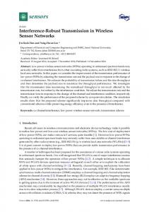
Fig. 2. An example of how concurrent transmissions are implicitly achieved in our work shows two nodes transmitting simultaneously to a receiver. Sniffer co-located with the transmitters record their corresponding transmitter’s packets. These packets are later analyzed to find which pair of packets is really concurrent by comparing their timestamps. An example timeline is shown, where back-to-back packets are transmitted with a slight jitter. Some packets undergo collisions at the receiver. Post-processing on the traces captured by sniffers 1 and 2 give us concurrent packets. Analysis of the receiver trace reveals which of these packets are received correctly and which are lost.
ii. All transmissions are captured at the co-located sniffer and timestamped using a synchronous time base. All successful packet receptions are also captured at the receiver of each link and timestamped similarly. As we will show in Section III-B, the transmissions are somewhat jittery. Thus, some post-processing is needed. iii The captured traces at the sniffers are post-processed to determine the actual sets of transmissions that overlap with a pre-defined degree of overlap (50% in our experiments). These sets of transmissions are deemed ‘concurrent’4. All other transmissions are ignored. iv. Success or failure of each transmission from each set of concurrent transmissions is noted from the receiver trace. 802.11 frame sequence number is used in identifying frames. v. Finally, from the above data, the packet reception rate (PRR) statistics is computed over a large number of such sample concurrent transmissions for each link in the chosen activation set. Several technical details are important to understand how the above is achieved. We discuss these in the following subsection. Then, we will describe some validation experiments to support our techniques. A. Technical Details a) Obtaining synchronized clocks. The 802.11 cards in the network nodes are set up in ad hoc mode. The time synchronization function (TSF) in 802.11 automatically synchronizes the clocks in the interface cards. To ensure that sniffers also utilize TSF, they are also made to run the ad hoc mode on a virtual interface, in addition to running the monitor mode on the main interface. Note that we do not disable beacon transmissions that are needed for clock synchronization using TSF. Microseconds resolution TSF 4 For details regarding the capture phenomenon, look at the related work section for a discussion.
0.4 0.35 0.3 0.25 0.2 0.15 0.1 0.05 0
0.05 0.045 0.04
-40
-20
0
20
40
Fraction of Packets
Relative frequency
4
0.035 0.03 0.025 0.02 0.015 0.01
Sync error (us)
0.005 0
B. Experimental Validation We have validated a), b) and c) above experimentally to ensure that they indeed work satisfactorily. To validate a), we essentially evaluate how good the TSF time synchronization is on our testbed. To do this, we conduct the following experiment. Each node in the testbed is made to transmit alone and all the other nodes receive these transmissions. As usual, the transmitted frame is also captured at the sender’s sniffer. Each packet is uniquely identified by the MAC address and frame sequence number in all captured traces. Each packet’s receive timestamp on each receiver is compared to the same packet’s timestamp on the sender’s sniffer. Figure 3 shows the distribution of the synchronization error (difference between these timestamps). Note the sharp peak at zero. Median error is 2 µs for the absolute difference. Note that this time is very small compared to the average packet transmission time in our experiments (2089 µs). We also validate b) and c), i.e., that the disabling of carriersense and backoff is working well. We perform an experiment where two network nodes concurrently transmit back-to-back UDP packets (size 1470 bytes) thus generating saturated loads. The nodes are kept within perfect carrier sense distance. The corresponding sniffers captures all transmissions from the senders. We observe that when carrier-sense and backoff are not disabled, the two senders share the medium and the aggregated transmit rate is 5.7Mbps, where one is 2.5 Mbps
Inter-Packet Time Difference (us)
(a) Carrier-sense, ACK and backoff enabled.
0.5 0.45 0.4 Fraction of Packets
timestamps are recorded in all captured frames in the sniffers or the receivers from the radiotap header. Thus, all captured frames in the network have a common time base (TSF time). This is useful for step iii above. b) Disabling carrier-sense. To achieve this we used the antenna switching technique [14]. The 802.11 interface uses two antenna connectors for diversity. We have only one antenna connected to one connector, keeping the other connector unconnected. Using driver-level commands, any one of the connector can be selected as the receiving/transmit antenna. Selecting the unconnected antenna as the receiving antenna effectively disables carrier sense. This is useful for step i above. c) Disabling backoffs. This is again achieved via driver-level commands by explicitly setting the initial backoff window size to zero and disabling retransmissions. Thus, there is only one transmission attempt with no backoff. The transmitted packets are MAC layer broadcasts; there are no ACKs.
21 72 21 82 21 93 22 09 22 19 22 28 22 39 22 53 22 65 22 75 22 89 22 98 23 10 > 25 00
Fig. 3. Distribution of the synchronization error (difference between the recorded timestamps at the sniffer and at the receivers for the same packet).
0.35 0.3 0.25 0.2 0.15 0.1 0.05 0 2088
2089
2106
2107
> 2500
Inter-Packet Time Difference (us)
(b) Carrier-sense, ACK and backoff disabled. Fig. 4. Distribution of inter-packet times (difference between start-time of successive packets) at the sniffers for two scenarios. Note packet time is 2089µs.
and the other is 3.2 Mbps (as per the captured packets at the sniffers). When carrier-sense and backoff are disabled, each sender transmit at 5.55 Mbps, almost doubling the aggregate sending rate. We also analyze the inter-packet times in the above experiment from the ‘merged’ packet trace captured at the sniffers as another form of validation. Their distributions are shown in Figure 4. Note 16 distinct peaks of inter-packet times without disabling carrier sense, ACK and backoff (denoting 16 possible backoff values in 802.11a). When they are disabled, we get two peaks with one corresponding to the packet time. There are also two other smaller peaks. We attribute the occurrence of these peaks to synchronization error, occasional beacon transmissions, hardware imperfections and unexplained software delays, or even occasional carrier-sensing directly from the antenna connector itself. Note also that in both cases a small fraction of packets have very high delay. These are clubbed together in the plot as their values take a very wide range. All these jitters are the reason why we do not rely on the scheduling system to be able to make perfect concurrent transmissions. This is also the reason post-processing is used to identify what sets of packets are really concurrent. IV. B UILDING AND E VALUATING P HYSICAL I NTERFERENCE M ODEL The physical interference model describes the success probability of a transmission (modeled in terms of packet reception rate or PRR) when one or more interferers are contributing to the interference at the receiver of the intended transmission. If S is the signal power received at the intended receiver from the sender, N is the noise power at the receiver and ΣI is
5
100
80
PRR
60
40
20 SINR vs PRR Fitted Curve
0 0
Fig. 5.
5
10
15 20 SINR (dB)
25
30
35
PRR vs. SINR relationship from measurement data.
the sum of the interference powers experienced at the receiver caused by the group of interferers (transmitting concurrently), the model predicts the relationship between the bit error rate S (BER) and SINR, where SINR = ΣI+N . This relationship depends on radio properties such as modulation. The packet error rate (PER) is directly related to BER and depends on coding. The packet reception rate (PRR), a quantity we will evaluate directly, is simply 1 − PER and thus again is directly related to SINR. Typically, the PRR vs. SINR curve makes a sharp transition from low to high PRR values with increasing SINR. The rising part of the function has been described as the transition region in [15], albeit for a different radio technology. Since scheduling applications need a ‘binary’ model (see, e.g., [6]), the curve is typically ‘thresholded’ and is described as a step function changing from 0 and 1 at a specific value of SINR, called the SINR threshold or capture threshold. This variant of the physical model is henceforth referred to as thresholded physical interference model. The original model will be called the graded physical interference model. A. Model Building To build the physical model, one needs to find the PRR vs. SINR relation. We do this empirically by simply taking many measurement samples of S, I and N for a separate three node setup – sender, receiver and interferer, thus directly computing S SINR as I+N . PRR is measured by noting the fraction of packets received at the receiver when the sender and interferer transmit concurrently. The above three node measurements use identical hardware and measurement mechanism as described in Sections II and III. This means that each node is accompanied by a sniffer, and concurrent transmissions are identified by postprocessing captured packet traces. To derive a statistically meaningful relationship between PRR and SINR, many different samples of are needed. We change the distances between transmitter-receiver and interferer-receiver pairs as well as change the transmit powers so that S and I can vary over a wide range. For each distances and transmit power setting (i.e., constant S and I), several thousands concurrent transmissions are used to compute PRR. This provides one sample. The samples are shown in the scatterplot in Figure 5. We also show a fitted curve using a linear interpolation of average values
in buckets of 1 dB each. This fitted curve provides the PRR vs. SINR model that will beused in our later analysis. This model can also be used directly by a scheduling algorithm. PRR is close to zero for SINRs less than about 10 dB and close to 100% for SINR more than about 25 dB. The transition region is thus quite wide. Note many intermediate PRRs are possible in the range of 15-22 dB. These considerations are important in choosing a topology for our study as discussed in Section II. Note that measurements on large mesh testbeds have shown significant number of intermediate level links. See, e.g., evaluations on MIT roofnet in [16] or Rice University testbed in [17]. B. Model Evaluation Our goal now is to evaluate the accuracy of the physical model for transmission scheduling. In particular, we will compare the two versions of physical model here – graded and thresholded, and also the thresholded model for different SINR thresholds. Since scheduling essentially determines ‘feasible’ activation sets (set of links) in each slot subject to an interference model, a model’s responsibility is to describe which sets of links are feasible together and which are not. Any scheduling algorithm must avoid the so-called primary interference, i.e., interference between links with a common endpoint in the network graph. Thus, the algorithm must choose a matching5 on the network graph as we are only considering unicast transmissions. Thus, instead of using random subset of links, we use random matchings. There is no point in evaluating non-matchings as they will never be scheduled by any algorithm. Choosing random matchings is intractable as well. We resort to a simple heuristics (not described here for brevity) to pick random matchings. It is important to define which are actually links in our mesh testbed. We assume that for each ordered pair of nodes A, B, there is a network link from node A to node B if transmissions from A to B have 90% or more PRR in the absence of any interference. While we would have liked to use a higher PRR threshold, this also reduces the number of concurrently usable links. Note from Figure 5 that very high PRR (95% or beyond) is rare in the testbed. 566 random matchings are used providing significant data sets. Such large data set also makes the study relatively independent of the topology used. This is because the data set includes many instances of links well distributed over the relevant range of SINR values. See Figure 1 again. For each randomly selected matching, the actual throughput (normalized) of each link is evaluated when all links in the matching are transmitting concurrently in the testbed. The normalized throughput is simply the number of packets received on each link divided by the number of packets transmitted on this link. The method described earlier in Section II is used to find concurrent transmissions and throughput is calculated over only those packets which are actually concurrent. For 5 A matching is a set of links such that no two links have a common end point.
6
100
model is much more accurate than the thresholded model in predicting the accuracy of scheduling. There is a slight difference in choice of threshold too. Note, however, this issue is actually a problem for the thresholded model, as the right threshold to use is not easy to determine in a practical set up. The CDF of actual error shows whether a model is biased towards under or over-estimation of expected throughput. In Figure 6(a), the thresholded model is clearly underestimating throughput – a sign of overly conservative modeling. This is expected as the thresholded model allows links to be scheduled only with high probability of success. The graded model, on the other hand, is relatively unbiased.
Percentage of links
80 60 40 20
Graded Thresholded (22.5 dB) Thresholded (25.0 dB)
0 -1
-0.5
0
0.5
1
Error
(a) Actual error. 100
V. E VALUATING S CHEDULING P ERFORMANCE
90 Percentage of links
80 70 60 50 40 30 20
Graded Thresholded (22.5 dB) Thresholded (25.0 dB)
10 0 0
0.2
0.4 0.6 Error
0.8
1
(b) Absolute error. Fig. 6. models.
CDF of modeling errors for thresholded and graded interference
each matching, about 3000 concurrent transmissions in the matching are used to calculate throughput. Each random matching is used as input to a predictor that evaluates the link throughput predicted by each interference model. For the thresholded model, the throughputs of all links in a matching that have above-threshold SINR are assumed to be 1. The rest are assumed to be 0. For the graded model, the throughputs are simply the PRRs as determined by the PRR vs. SINR relation (Section IV). The modeling error is evaluated in the following fashion. Given a matching Mi consisting of |Mi | links we denote the measured throughput for j-th link in this matching as Γji (measured) and the predicted throughput by model k as Γji (model). Then the modeling error with respect to the j-th link in the matching Mi is given by errorij (model) = Γji (measured) − Γji (model).
(1)
The cumulative distribution function (CDF) of the modeling errors (Equation 1) is plotted in Figure 6. Errors for the graded and thresholded versions of the physical model are shown separately. Two different thresholds are used for the thresholded model 25 dB and 22.5 dB to demonstrate the impact of choice of threshold. Figure 6(a) shows the CDF of actual modeling error while Figure 6(b) shows the CDF of absolute error. Out of the evaluated links, 50 percent links show an absolute error below 0.05 for graded model and 0.2 for the thresholded model. The 80 percentile absolute error is in fact much lower for graded model (0.2) and very high for the thresholded model (0.5–0.6). This shows that the graded
The previous section evaluated the accuracy of the two incarnations of the interference models in predicting the feasibility of a randomly chosen set of links. These evaluations only focus on modeling accuracy, but do not directly model real performances when used in a scheduling algorithm. This is because a scheduling algorithm considers only specific subsets of feasible links. This is entirely algorithm dependent. To gain some insight here, we now study the performances of the two physical interference models for making actual scheduling decisions. To do this, however, we need to use scheduling algorithms. One concern here is that the two interference models behave quite differently. The thresholded model is binary, while the graded model is not. In our knowledge, all scheduling algorithms in literature deal with binary models and not with probabilistic models. However, using probabilistic models directly in scheduling has potential for improved throughput. This has been partially addressed by the model accuracy evaluation in the previous section, where it has been shown that the thresholded model can be overly conservative. It only allows transmissions with very high (close to 100%) probability of success. Can we gain extra capacity by allowing transmissions with less than perfect success probability? Note that extra capacity could be substantial if there are many links in the transition region. To address this question we need to develop new scheduling algorithms that can treat links as nonbinary. A comprehensive treatment of this topic is beyond the scope of this paper. Here, we want to focus on measurements only. To demonstrate the potential of the graded model in scheduling we use a two-part approach: • In the first part, we study the two models using the greedy scheduling algorithm. Greedy scheduling has often been considered in literature – both for physical (thresholded) [6] and other simpler interference models [18], [19]. The goal there has been primarily to investigate its optimality properties. We extend greedy scheduling to the graded model; though its performance bound remains unknown. • In the second part, we use optimal scheduling using both models. Since optimal algorithms for either model for the general scheduling problem are open questions, we use a
7
Fig. 7. Results of greedy scheduling showing measured aggregate throughput for thresholded and graded physical models for different link demand vectors.
simplified scheduling problem (one-shot scheduling [20]) here. The advantage here is that exhaustive searches are possible to determine the optimal for small networks such as ours. The following two subsections describe these two parts respectively. A. Scheduling Using Greedy Algorithm We use the same greedy scheduling algorithm for both models. It is straightforward to implement and performance bounds are known for specific models, including the thresholded version of physical model [6], [18], [21]. The link demand vector is an input to the algorithm. The demand for a link is simply the number of packets (each packet takes one slot to transmit) to be scheduled on the link. The schedule is a sequence of slots with a feasible set of links to be scheduled in each slot such that demands of all links are satisfied. This is sometimes called the evacuation model. We describe the greedy algorithm below for a binary interference model (thresholded physical model in our case). We will describe later how it is modified to run under the graded model. Input: Network graph G = (V, E), demand vector on the links f = (f1 , . . . , f|E| ) and the interference model. The interference model specifies which set of links (activation sets) are ‘feasible’ together. Output: Schedule S = {S1 , S2 , . . . , Sτ }, where Sk is a feasible set of links scheduled in the same slot. τ is the schedule length. Algorithm: 1) Order and rename links such that f1 ≥ f2 ≥ f3 . . . ≥ f|E| . 2) Set i = 1, S = φ, τ = 0. (Initial schedule is empty.) 3) Schedule link i in the very first available slot where it can be scheduled interference-free according to the given interference model. If no such slot of feasible, increment τ and schedule the link in the last slot. (Incrementing τ is equivalent to creating a new empty slot at the end of the current schedule.) 4) Repeat step 3 above fi times. 5) Increment i. Go back to step 3 until i > |E|. For non-binary models such as the graded model, the algorithm is modified as follows. There is no real notion of
feasibility now. Any set of links can be scheduled together, providing probabilistic packet deliveries on the constituent links. Thus, we use the notion of expected throughput in a slot to design the greedy algorithm. The expected throughput is the sum of the PRRs in all scheduled links per the PRR vs. SINR relation defining the interference model. In the greedy choice step above (step 3), the link i is scheduled in the first available slot so that its addition to that slot does not decrease the expected throughput in that slot. The two models are compared in the following fashion. Four different demand vectors are considered for experiments, 1 through 4. The links are split into two equal sets randomly. One set has one packet each. The other set has i packets each for vector i. The models generate different schedules for a given demand vector. The schedules generated by each model are evaluated using scheduling experiments on the testbed. Each slot in the schedule is an activation set and concurrent transmissions are scheduled and identified in the same way as described in Section III by sending 3000 back-to-back packets transmitted on all links in the activation set concurrently. As outlined in that section, only actual concurrent packets are used for calculating the reception rate at the receiver on a link. This gives us the throughput on each link in a slot. All slots are evaluated for throughput in the same manner. Throughput is measured for each slot in number of packets per slot and is averaged for the entire schedule. The results are presented in Figure 7. The results show that graded model consistently gives higher throughput than the thresholded models (for either threshold). On an average, the percentage improvement of graded model against thresholded model with SINR threshold of 22.5 dB is 56% and with SINR threshold of 25.0 dB is 74%. This demonstrates the potential of using the graded model directly in scheduling. B. One Shot Scheduling One limitation of the above study is that while the same greedy scheduling is used for both models, it remains inconclusive regarding why the graded model is performing better. Is it due to a better modeling accuracy or due to a better algorithm? While the performance bound for the greedy algorithm for the thresholded model is known, it is quite loose [6]. Also, the bound for the graded is unknown. Thus, we do not have any useful tool to answer this question. So, in order to make our observations stronger, we study a simplified scheduling problem called “One Shot Scheduling” [20], where we can reasonably implement optimal algorithms for both models. Thus, only modeling accuracy will play any role. The one shot scheduling problem picks a subset S of links to be scheduled from a given set L such that the aggregate throughput is maximized. We redefine throughput as ‘expected throughput’ as we are dealing with probabilistic transmission success. The one shot scheduling problem for the thresholded physical model has been shown to be intractable [20]. But, for small size of L, it is computationally feasible to exhaustively
8
Fig. 8.
Results of the One Shot Scheduling experiment comparing the thresholded and graded physical models.
look for the optimal subset Sopt to be scheduled. Any set of schedulable links has to be a matching. Thus, we can preselect L as a matching. With a 11 node network |L| is upperbounded by 5. Thus, exhaustive search is feasible to obtain optimal schedules for both models. One needs to evaluate only 31 possibilities. The experiments are done as follows. First, we obtain the connectivity graph of the network. We again define network links as those with PRR greater than 90% in absence of any interference. For each experiment, we pick a random matching L from the connectivity graph such that the |L| is equal or close to 5. For each model, we estimate the throughput of each subset S of L and then choose the optimal subset Sopt which provides the maximum aggregate throughput. Note that the Sopt for the graded model can be different than Sopt for the thresholded model. Thus, for each experiment, we schedule both these subsets one by one in the testbed to find their respective throughputs. The same method as used earlier in greedy scheduling (described in Section III) is used to schedule concurrent transmissions. We also determine the aggregate throughput for each subset using the same method as used before. We perform 84 such experiments with different random choice of L each time. Due to lack of space, results for randomly chosen 30 experiments (out of the 84) are shown in Figure 8. Throughput is expressed in terms of average number of packets successfully transmitted per slot. This is the Y-axis. The individual experiments (i.e., different choices of L) are shown on the Xaxis, sorted in the order of increasing throughput for the graded model for visual clarity. For each experiment, the throughput for graded model is drawn as a bar graph on the left and the throughputs for thresholded models are drawn as a bar graphs on its left. In all experiments, graded model gives higher throughput. Overall (for all 84 experiments), the graded model improves throughput per slot by 77% over the thresholded model with threshold of 22.5 dB and by about 146% over the thresholded model with threshold of 25.0 dB. Note again choosing the right threshold is tricky with extensive experiments. This simple one shot scheduling experiment again establishes the power of using graded physical interference model instead of using the more conventional thresholded model for use in scheduling.
VI. R ELATED W ORK Interference modeling using the physical model or promoting the use of such models have been the topic of several recent 802.11-based empirical modeling and evaluation work. However, these are based on the default CSMA/CA MAC protocol of 802.11 and part of their effort goes into modeling the carrier-sense aspects and how transmission capacity is shared. In [22], authors investigated the impact of carrier sensing. In [23], Padhye et. al. developed a measurementbased methodology to characterize link interference in 802.11 networks. They pointed out that interference between links is not “binary” in practice. In [24], the authors showed that pairwise interference modeling is often not accurate and multiple interferers must be accounted for. Techniques for generating interference maps have been developed in [25]. Measurementbased modeling to evaluate 802.11 link capacities have been used in [26]–[28]. We also use measurement-based modeling, albeit for a different goal. Several papers also studied capture effects on 802.11 with different modulations (802.11b and 802.11a) and chipsets [29]–[32]. Experience with the capture model varied somewhat depending on the actual technology used. This varied from scenarios, where the second packet out of two overlapping packets cannot be captured if it arrives after the preamble period of the first packet, to cases where it can be captured when the MIM (message-in-message) mode [31], [32] is implemented. Note that we consider 50% overlapped of packets as concurrent and do not give any special consideration for first or second packet. The reason for this is that independent analysis revealed no statistical difference of the capture behavior for the first or second packet, likely because MIM is implemented in the Atheros chipset we use. TDMA-based MAC on commodity 802.11 hardware has been a topic of several investigations [4], [5], [13], [14]. None of these, however, directly address the interference modeling question. However, they do address many implementation issues that are perfectly complimentary to our goal. We do note that synchronization achieved by software-level implementations in these papers are not tight enough to have one packet per slot at the data rate we use. Roughly, slot sizes in the order of 10ms have been achieved, while our packet time is about 2ms in this paper. However, future firmware level developments are expected to address these limitations. Moving over to non-802.11 platforms, evaluations similar
9
to this paper are available. Concurrent transmissions on lowpower sensor motes have been studied in [15], [33], [34]. Our recent works [35], [36] on motes platforms also studied interference modeling aspects. Some of the approaches used in the current paper are similar to those we used in [36]. Note that TDMA-based scheduling in mote-class radios such as 802.15.4 is easier to achieve as the radios are better documented than 802.11 radios and data rates are much slower. VII. C ONCLUSIONS
AND
F UTURE D IRECTIONS
Our work makes the following contributions. First, we evaluate the accuracy of physical interference modeling on an 802.11a testbed. We show that the thresholded model commonly used for scheduling has much poorer accuracy relative to the graded model that we promote for scheduling use. The graded model is not perfect, however. The 80 percentile error is 0.2 (normalized to maximum link throughput 1 packet/slot). Second, we show using two types of scheduling experiments that the accuracy question hurts the performance of the thresholded model badly. The graded model achieves a better throughout by a factor of roughly 2. This stems primarily from the overly conservative behavior of the thresholded model that schedules perfect links only. Our recommendation for future work is thus to embrace the reality and investigate scheduling algorithms that exploit the graded model for creating highperformance mesh backbones using 802.11. A careful reader will note that a physical layer rate reduction would improve PRR for a given SINR. One can argue that the thresholded model can always be used if the rate can be adjusted to obtain a high enough PRR for the available SINR. While this is true, standardized protocols and hardwares allow rate adjustments with only a very course granularity (e.g., only a few available rates in 802.11). Also, many mesh networks may use long distance links [13] and may thus operate at the lowest possible rate. Thus, our approach of scheduling imperfect links is still very useful. A comprehensive study of rate control along with scheduling imperfect links is also an important direction for future work. R EFERENCES [1] A. P. Jardosh, K. N. Ramachandran, K. C. Almeroth, and E. M. BeldingRoyer, “Understanding congestion in ieee 802.11b wireless networks,” in ACM IMC, 2005. [2] M. Rodrig, C. Reis, R. Mahajan, D. Wetherall, and J. Zahorjan, “Measurement-based characterization of 802.11 in a hotspot setting,” in ACM E-WIND, 2005. [3] M. Garetto, T. Salonidis, and E. W. Knightly, “Modeling per-flow throughput and capturing starvation in csma multi-hop wireless networks,” in Proc. of IEEE INFOCOM, Barcelona, April 2006. [4] M. Neufeld, J. Fifield, C. Doerr, A. Sheth, and D. Grunwald, “Softmacflexible wireless research platform,” in In Proc. HotNets-IV, Nov 2005. [5] A. Rao and I. Stoica, “An overlay MAC layer for 802.11 networks,” in ACM MobiSys’05, 2005, pp. 135–148. [6] G. Brar, D. M. Blough, and P. Santi, “Computationally efficient scheduling with the physical interference model for throughput improvement in wireless mesh networks,” in MobiCom ’06, 2006. [7] J. Gronkvist and A. Hansson, “Comparison between graph-based and interference-based STDMA scheduling,” in MobiHoc, 2001. [8] T. Moscibroda and R. Wattenhofer, “The complexity of connectivity in wireless networks,” in IEEE INFOCOM, 2006.
[9] P. Gupta and P. R. Kumar, “The capacity of wireless networks,” IEEE Transactions on Information Theory, vol. 46, no. 2, pp. 388–404, March 2000. [10] D. Blough, S. R. Das, G. Resta, and P. Santi, “A framework for joint scheduling and diversity exploitation under physical interference in wireless mesh networks,” in IEEE MASS, Atlanta, 2008. [11] Soekris Engineering, http://www.soekris.com. [12] “HFA3863 Data Sheet: Direct Sequence Spread Spectrum Baseband Processor with Rake Receiver and Equalizer,” Intersil Corporation, 2000. [13] R. Patra, S. Nedevschi, S. Surana, A. Sheth, L. Subramanian, and E. Brewer, “WiLDNet: Design and Implementation of High Performance WiFi Based Long Distance Networks,” NSDI, 2007. [14] K. Chebrolu, B. Raman, and S. Sen, “Long-distance 802.11b links: Performance measurements and experience,” in ACM MobiCom, 2006. [15] M. Zuniga and B. Krishnamachari, “Analyzing the transitional region in low power wireless links,” in IEEE SECON 2004, 2004, pp. 517–526. [16] D. Aguayo, J. Bicket, S. Biswas, G. Judd, and R. Morris, “Link-level measurements from an 802.11b mesh network,” in Proc. SIGCOMM 2004, 2004. [17] J. Camp, J. Robinson, C. Steger, and E. Knightly, “Measurement driven deployment of a two-tier urban mesh access network,” in Proc. ACM MobiSys, 2006, pp. 96–109. [18] G. Sharma, R. Mazumdar, and N. Shroff, “On the complexity of scheduling in wireless networks,” in Proc. ACM MobiCom, 2006. [19] X. Wu and R. Srikant, “Bounds on the capacity region of multi-hop wireless networks under distributed greedy scheduling,” in Proc. IEEE INFOCOM, 2006. [20] O. Goussevskaia, Y. A. Oswald, and R. Wattenhofer, “Complexity in geometric SINR,” in ACM MobiHoc’07, 2007, pp. 100–109. [21] H. Balakrishnan, C. L. Barrett, V. S. A. Kumar, M. V. Marathe, and S. Thite, “The distance-2 matching problem and its relationship to the MAC-layer capacity of ad hoc networks,” IEEE J. Selected Areas of Communication, pp. 1069–1079, 2004. [22] K. Jamieson, B. Hull, A. K. Miu, and H. Balakrishnan, “Understanding the Real-World Performance of Carrier Sense,” in E-WIND, Philadelphia, PA, August 2005. [23] J. Padhye, S. Agarwal, V. Padmanabhan, L. Qiu, A. Rao, and B. Zill, “Estimation of link interference in static multi-hop wireless networks,” in IMC, 2005. [24] S. Das, D. Koutsonikolas, Y. Hu, and D. Peroulis, “Characterizing multiway interference in wireless mesh networks.” in ACM WiNTECH, 2005. [25] D. Niculescu, “Interference map for 802.11 networks,” in Proc. IMC, 2007. [26] C. Reis, R. Mahajan, M. Rodrig, D. Wetherall, and J. Zahorjan, “Measurement-based models of delivery and interference in static wireless networks,” in ACM SIGCOMM, 2006. [27] A. Kashyap, S. Ganguly, and S. R. Das, “A measurement-based approach to modeling link capacity in 802.11-based wireless networks,” in ACM MobiCom, 2007. [28] L. Qiu, Y. Zhang, F. Wang, M. K. Han, and R. Mahajan, “A general model of wireless interference,” in ACM MobiCom, 2007. [29] A. Kochut, A. Vasan, A. Shankar, and A. Agrawala, “Sniffng out the correct physical layer capture model in 802.11b,” in Proc. IEEE ICNP, Berlin, 2004. [30] H. Chang, V. Misra, and D. Rubenstein, “A general model and analysis of physical layer capture in 802.11 networks,” in Proc. IEEE Infocom, 2006. [31] J. Lee, W. Kim, S.-J. Lee, D. Jo, J. Ryu, T. Kwon, and Y. Choi, “An experimental study on the capture effect in 802.11a networks,” in Proc. ACM WiNTECH, 2007. [32] J. Ryu, J. Lee, S.-J. Lee, and T. Kwon, “Revamping the ieee 802.11a phy simulation models,” in Proceedings of ACM MSWiM, Vancouver, 2008. [33] D. Son, B. Krishnamachari, and J. Heidemann, “Experimental study of concurrent transmission in wireless sensor networks,” in SenSys ’06, 2006, pp. 237–250. [34] K. Whitehouse, A. Woo, F. Jiang, J. Polastre, and D. Culler, “Exploiting the capture effect for collision detection and recovery,” in IEEE EmNetSII, May 2005. [35] R. Maheshwari, S. Jain, and S. R. Das, “On estimating joint interference for concurrent packet transmissions in low power wireless networks,” in Proc. ACM WiNTECH, 2008. [36] ——, “A measurement study of interference modeling and scheduling in low-power wireless networks,” in Proc. ACM SenSys, 2008.