A Memetic Algorithm with Bucket Elimination for the Still Life Problem

A Memetic Algorithm with Bucket Elimination for the Still Life Problem Jos´e E. Gallardo, Carlos Cotta, and Antonio J. Fern´andez Dept. Lenguajes y Ciencias de la Computaci´ on, ETSI Inform´ atica, University of M´ alaga, Campus de Teatinos, 29071 - M´ alaga, Spain. {pepeg,ccottap,afdez}@lcc.uma.es

Abstract. Bucket elimination (BE) is an exact technique based on variable elimination, commonly used for solving constraint satisfaction problems. We consider the hybridization of BE with evolutionary algorithms endowed with tabu search. The resulting memetic algorithm (MA) uses BE as a mechanism for recombining solutions, providing the best possible child from the parental set. This MA is applied to the maximum density still life problem. Experimental tests indicate that the MA provides optimal or near-optimal results at an acceptable computational cost.

1

Introduction

The game of life [1] consists of an infinite checkerboard in which the only player places checkers on some of its squares. Each square is a cell that has eight neighbors: the eight cells that share one or two corners with it. A cell is alive if there is a checker on it, and dead otherwise. The state of the board evolves iteratively according to three rules: (i) if a cell has exactly two living neighbors then its state remains the same in the next iteration, (ii) if a cell has exactly three living neighbors then it is alive in the next iteration and (iii) if a cell has fewer than two or more than three living neighbors, then it is dead in the next iteration. An interesting extension of this game is the maximum density still life problem (MDSLP) that consists of finding board configurations with a maximal number of living cells not changing along time. These stable configurations are called maximum density stable patterns or simply still lifes. In this paper we are concerned with the MDSLP and finite patterns, i.e., finding n × n still lifes. No polynomial method is known for this problem. Our interest in this problem is manifold. Firstly, it must be noted that the patterns resulting in the game of life are very interesting. For example, by clever placement of the checkers and adequate interpretation of the patterns, it is possible to create a Turing-equivalent computing machine [2]. From a more applied point of view, it is interesting to consider that many aspects of discrete dynamical systems have been developed or illustrated by examples in life game [3, 4]. In this sense, finding stable patterns can be regarded as a mathematical abstraction of a standard issue in discrete systems control. Finally, the MDSLP is a prime example of weighted constrained optimization problem, and as such constitutes an excellent test bed for different optimization techniques.

The still life problem has been recently included in the CSPLib repository and a dedicated web page1 maintains up-to-date results. This problem has been tackled using different approaches. Bosch and Trick [5] used a hybrid approach mixing integer programming and constraint programming to solve the cases for n = 14 and n = 15 in about 6 and 8 days of CPU time respectively. Smith [6] considered a pure constraint programming approach to tackle the problem and proposed a formulation of the problem as a constraint satisfaction problem with 0-1 variables and non-binary constraints. A dual formulation of the problem was also considered, and it was proved that this dual representation outperformed the initial one (although it could only solve instances up to n = 10). In any case, this dual encoding was particularly useful to find (90◦ rotational) symmetric solutions (e.g., it found the optimal solution for n = 18). Later on, Larrosa et al. [7, 8] showed the usefulness of variable elimination techniques, namely bucket elimination (BE), on this problem. Their basic approach could solve the problem for n = 14 in about 105 seconds. Further improvements pushed the solvability boundary forward to n = 20 in about the same time. At any rate, it is clear that these exact approaches are inherently limited for increasing problem sizes, and their capabilities as anytime algorithms are unclear. Furthermore, to the best of our knowledge no heuristic approaches to this problem have been attempted. In this work, we consider the hybridization of evolutionary algorithms with the BE approach. We will show that memetic algorithms (MAs) endowed with BE can provide optimal or near-optimal solutions at an acceptable computational cost. To do so, we will firstly introduce the essentials of BE in next section.

2

WCSPs and Bucket Elimination

A Weighted constraint satisfaction problem (WCSP) [9] is a constraint satisfaction problem (CSP) in which the user can express preferences among solutions. A WCSP is defined by a tuple (X, D, F ), where X = {x1 , · · · , xn } is a set of variables taking values from their finite domains (Di ∈ D is the domain of xi ) and F is a set of cost functions (also called soft constraints). Each f ∈ F is defined over a subset of variables var(f ) ⊆ X, called its scope. For each assignment t of all variables in the scope of a soft constraint f , t ∈ f (i.e., t is permitted) if, and only if, t is allowed by the soft constraint. A complete assignment that satisfies every soft constraint represents a solution to the WCSP. The valuation of an assignment t is defined as the sum of costs of all functions whose scope is assigned by t. Permitted assignments receive finite costs that express their degree of preference and forbidden assignments receive cost ∞. The optimization goal consists of finding the solution with the lowest valuation. 2.1

The Bucket Elimination Approach

Bucket elimination [10] is a generic algorithm suitable for many automated reasoning and optimization problems, in particular for WCSP solving. 1

http://www.ai.sri.com/∼nysmith/life/

1: 2: 3: 4: 5: 6: 7: 8: 9: 10: 11:

function BE(X, D, F ) for i := n downto 1 do Bi := {f ∈ F | xi ∈ var(f )} P gi := ( f ∈Bi f ) ⇓ i S F := (F {gi }) − Bi end for t := ∅ for i := 1 to n do P v := argmina∈Di {( f ∈Bi f )(t · (xi , a))} t := t · (xi , v) end for return(F, t) end function Fig. 1. The general template of Bucket Elimination for a WCSP (X, D, F ).

BE is based upon the following two operators over functions: – The sum of two functions f and g denoted (f + g) is a new function with scope var(f ) ∪ var(g) which returns for each tuple the sum of costs of f and g defined as (f + g)(t) = f (t) + g(t); – The elimination of variable xi from f , denoted f ⇓ i, is a new function with scope var(f ) − {xi } which returns for each tuple t the minimum cost extension of t to xi , defined as (f · i)(t) = mina∈Di {f (t · (xi , a))} where t · (xi , a) means the extension of t to the assignment of a to xi . Observe that when f is a unary function (i.e., arity one), eliminating the only variable in its scope produces a constant. Fig. 1 shows an operational schema of the BE algorithm for solving a certain WCSP. The displayed algorithm returns the optimal cost in F and one optimal assignment in t. Note that BE has exponential space complexity because in general, the result of summing functions or eliminating variables cannot be expressed intensionally by algebraic expressions and, as a consequence, intermediate results have to be collected extensionally in tables. As it can be seen in Fig. 1, BE works in two phases. In the first phase (lines 1-5), the algorithm eliminates variables one at a time in reverse order according to an arbitrary variable ordering o (without loss of generality, here we assume lexicographical ordering for the variables in X, i.e, o = (x1 , x2 , · · · , xn )). In the second phase (lines 6-10), the optimal assignment is computed processing variables in increasing order. The elimination of variable xi is done as follows: initially (line 2), all cost functions in F having xi in their scope are stored in Bi (the so called bucket of xi ). Next (line 3), BE creates a new function gi defined as the sum of all functions in Bi in which variable xi has been eliminated. Then (line 4), this function is added to F that is also updated by removing the functions in Bi . The consequence is that the new F does not contain xi (all functions mentioning xi were removed) but preserves the value of the optimal

cost. The elimination of the last variable produces an empty scope function (i.e., a constant) which is the optimal cost of the problem. The second phase (lines 6-10) generates an optimal assignment of variables. It uses the set of buckets that were computed in the first phase: starting from an empty assignment t (line 6), variables are assigned from first to last according to o. The optimal value for xi is the best value regarding the extension of t with respect to the sum of functions in Bi (lines 8,9). We use argmina {f (a)} to denote the value of a producing minimum f (a). The complexity of BE depends on the problem structure (as captured by its constraint graph G) and the ordering o. According to [8], the complexity of BE ∗ ∗ along ordering o is time Θ(Q × n × dw (o)+1 ) and space Θ(n × dw (o) ), where d is the largest domain size, Q is the cost of evaluating cost functions (usually assumed Θ(1)), and w∗ (o) is the maximum width of nodes in the induced graph of G relative to o (check [8] for details). 2.2

Bucket Elimination for the Still Life Problem

The general template presented above can be readily applied to the MDSLP. To this end, let us first introduce some notation. A board configuration for a n×n instance will be represented by a n-dimensional vector (r1 , r2 , . . . , rn ). Each vector component encodes (as a binary string) a row, so that the j-th bit of row ri (noted rij ) indicates the state of the j-th cell of the i-th row (a value of 1 represents a live cell and a value of 0 a dead cell). Let Zeroes(r) be the number of zeroes in binary string r and let Adjacents(r) be the maximum number of adjacent living cells in row r. If ri is a row and ri−1 and ri+1 are the rows above and below r, then Stable(ri−1 , r, ri+1 ) is a predicate satisfied if, and only if, all cells in r are stable. The formulation has n cost functions fi (i ∈ {1..n}). For i ∈ {2..n − 1}, fi is ternary with scope var(fi ) = {ri−1 , ri , ri+1 } and is defined as2 :  ∞ : ¬Stable(a, b, c)    ∞ : a1 = b1 = c1 = 1 fi (a, b, c) = (1) ∞ : an = bn = cn = 1    Zeroes(b) : otherwise As to f1 , it is binary with scope var(f1 ) = {r1 , r2 } and is specified as:  ∞ : ¬Stable(0, b, c)  ∞ : Adjacents(b) > 2 f1 (b, c) =  Zeroes(b) : otherwise Likewise, the scope of fn is var(fn ) = {rn−1 , rn } and its definition is:  ∞ : ¬Stable(a, b, 0)  ∞ : Adjacents(b) > 2 fn (a, b) =  Zeroes(b) : otherwise 2

(2)

(3)

Notice in these definitions that stability is not only required within the pattern, but also in the surrounding cells (assumed dead).

1: 2: 3: 4: 5: 6: 7: 8: 9: 10: 11: 12: 13: 14: 15:

function BE(n, D) for a, b ∈ D do gn (a, b) := minc∈D {fn−1 (a, b, c) + fn (b, c)} end for for i := n − 1 downto 3 do for a, b ∈ D do gi (a, b) := minc∈D {fi−1 (a, b, c) + gi+1 (b, c)} end for end for (r1 , r2 ) := argmina,b∈D {g3 (a, b) + f1 (a, b)} opt := g3 (r1 , r2 ) + f1 (r1 , r2 ) for i := 3 to n − 1 do ri := argminc∈D {fi−1 (ri−2 , ri−1 , c) + gi+1 (ri−1 , c)} end for rn := argminc∈D {fn−1 (rn−2 , rn−1 , c) + fn (rn−1 , c)} return (opt, (r1 , r2 , . . . , rn )) end function Fig. 2. Bucket Elimination for the MDSLP.

Due to the sequential structure of the corresponding constraint graph, the model can be easily solved with BE. Fig. 2 shows the corresponding algorithm. Function BE takes two parameters: n is the size of the instance to be solved, and D is the domain for each variable (row) in the solution. If domain D is set to {0..2n − 1} (i.e., a set containing all possible rows) the function implements an exact method that returns the optimal solution for the problem instance (as the number of dead cells) and a vector corresponding to rows representing that solution. Note that the complexity of this method is time Θ(n2 × 23n ) and space Θ(n × 22n ). On the other hand, a basic search-based solution to the problem 2 could be implemented with worst case time complexity Θ(2(n ) ) and polynomial space. Observe that the time complexity of BE is therefore an exponential improvement over basic search algorithms, although its high space complexity makes the approach unpractical for large instances.

3

A Memetic Algorithm for the MDSLP

WSCPs are very amenable for being tackled with evolutionary metaheuristics. The quality of the results will obviously depend on how well the structure of the soft constraints is captured by the search mechanisms used in the optimization algorithm. To this end, problem-aware algorithmic components are essential. In the particular case of the MDSLP, we will use tabu search (TS) and BE for this purpose, integrating them into a memetic approach. Before detailing these two components, let us describe the basic underlying evolutionary algorithm (EA).

3.1

Representation and Fitness Calculation

The natural representation of MDSLP solutions is the binary encoding. Configurations will be represented as a binary n × n matrix r. Clearly, not all such binary matrices will correspond to stable patterns, i.e., infeasible solutions can be represented. We have opted for using a penalty-based fitness function in order to deal with such infeasible solutions. To be precise, the fitness (to be minimized) of a configuration r is computed as: f (r) = n2 −

n X n X

rij + K

i=1 j=1

n+1 X n+1 X

£ 0 ¤ 0 rij φ1 (ηij ) + (1 − rij )φ0 (ηij )

(4)

i=0 j=0

where r0 is an (n+2)×(n+2) binary matrix obtained by embedding r in a frame 0 0 of dead cells (i.e., rij = rij for i, j ∈ {1..n}, and rij = 0 otherwise – recall that stability is not only required within the n × n board, but also in its immediate neighborhood), K is a constant, ηij is the number of live neighbors of cell (i, j), and φ0 , φ1 : N −→ N are two functions defined as:  ½ if 2 6 η 6 3 0 0 if η 6= 3 if η < 2 φ0 (η) = φ1 (η) = K 0 + 2 − η (5) 0 K + 1 otherwise  0 K +η−3 if η > 3 where K 0 is another constant. The first double sum in Eq. (4) corresponds to the basic quality measure for feasible solutions, i.e., the number of active cells. As to the last term, it represents the penalty for infeasible solutions. The strength of penalization is controlled by constants K and K 0 . We have chosen K = n2 and K 0 = 5n2 . With this setting, given any two solutions r and s, the one that violates less constraints is preferred; if two solutions violate the same number of constraints, the one whose overall degree of violation (i.e., distance to feasibility) is lower is preferred. Finally, if the two solutions are feasible, the penalty term is null and the solution with the higher number of live cells is better. 3.2

A Local Improvement Strategy Based on Tabu Search

The fitness function defined above provides a stratified notion of gradient that can be exploited by a local search strategy. Moreover, notice that the function is quite decomposable, since interactions among variables are limited to adjacent cells in the board. Thus, whenever a configuration is modified, the new fitness can be computed just considering the cells located in adjacent positions to changed cells. To be precise, assume that cell (i, j) is modified in solution r, resulting in solution s; the new fitness f (s) can be computed as:  f (s) = f (r) + K ∆f1 (rij , ηij ) +

 X i0 ,j 0

∆f2 (ri0 j 0 , ηi0 j 0 , rij )

(6)

where the sum in the last term ranges across all cells (i0 , j 0 ) adjacent to (i, j), and functions ∆f1 and ∆f2 are defined as:  η=2 0 ∆f1 (c, η) = (−1)(1−c) φ0 (η) η = 3 (7)  (−1)c φ1 (η) otherwise ∆f2 (c0 , η, c) = (1 − c0 )∆f2,0 (η, c) + c0 ∆f2,1 (η, c)  0 (η = 2 ∧ c = 0) ∨ (η = 4 ∧ c = 1) K + 1 ∆f2,0 (η, c) = −(K 0 + 1) η = 3  0 otherwise  0 K +1 (η = 2 ∧ c = 1) ∨ (η = 3 ∧ c = 0)    0  −(K + 1) (η = 1 ∧ c = 0) ∨ (η = 4 ∧ c = 1)  (η = 1 ∧ c = 1) ∨ (η > 4 ∧ c = 0) ∆f2,1 (η, c) = 1   −1 (η = 0) ∨ (η > 5 ∧ c = 1)    0 otherwise

(8) (9)

(10)

Using this efficient fitness re-computation mechanism, our local search strategy explores the neighborhood N (r) = {s | Hamming(r, s) = 1}, i.e., the set of solutions obtained by flipping exactly one cell in the configuration. This neighborhood comprises n2 configurations, and it is fully explored in order to select the best neighbor. In order to escape from local optima, a tabu-search scheme is used: up-hill moves are allowed, and after flipping a cell, it is put in the tabu list for a number of iterations (randomly drawn from [n/2, 3n/2] to hinder cycling in the search). Thus, it cannot be modified in the subsequent iterations unless the aspiration criterion is fulfilled. In this case, the aspiration criterion is improving the best solution found in that run of the local search strategy. The whole process is repeated until a maximum number of iterations is reached, and the best solution found is returned. 3.3

Optimal recombination with BE

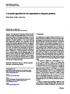
In the context of the fitness function that we have considered, the binary representation used turns out to be freely manipulable: any configuration can be evaluated, and therefore any standard recombination operator for binary strings could be utilized in principle. For example, we could consider the two-dimensional version of single-point crossover, depicted in Fig. 3. While feasible from a computational point of view, such a blind operator would perform poorly though: it would be more similar to macromutation than to a sensible recombination of information. To fulfill this latter goal, we can resort to BE. In section 2.2 it was shown how BE could be used to implement an exact method to solve the MDSLP. Although the resulting algorithm was better than basic search-based approaches, the corresponding time and space complexity were very high. In the following we describe how BE can be used to implement a recombination operator that explores the dynastic potential [11] (possible children) of the solutions being recombined, providing the best solution that can be constructed without introducing implicit mutation (i.e., exogenous information).

Random Column ↓

A1 Random Row

A2

B1

B2

×

→ A3

A4

A1

B2

B3

A4

= B3

B4

Fig. 3. Blind recombination operator for the MDSLP.

Let x = (x1 , x2 , · · · , xn ) and y = (y1 , y2 , · · · , yn ) be two board configurations for a n × n instance of the MDSLP. Then, BE(n, {x1 , x2 , · · · , xn , y1 , y2 , · · · , yn }) calculates the best feasible configuration that can be obtained by combining rows in x and y without introducing information not present in any of the parents. Observe that we are just restricting the domain of variables to take values corresponding to the configurations being recombined, so that the result of function BE is the best possible recombination. In order to analyze time complexity for this recombination operator, the critical part of the algorithm is the execution of lines 4-8 in Figure 2. In this case, line 6 has complexity O(n2 ) (finding the minimum of at most 2n alternatives, the computation of each being Θ(n)). Line 6 has to be executed n×2n×2n times at most, making a global complexity of O(n5 ) = O(|x|2.5 ), where |x| ∈ Θ(n2 ) is the size of solutions. Notice also that the recombination procedure can be readily made to further exploit the symmetry of the problem, extending variable domains to column values in addition to row values. The complexity bounds remain the same in this case. It must be noted that the described operator S can be generalized to recombine any number of board configurations like BE(n, x∈S {xi | i ∈ {1..n}}) where S is a set comprising the solutions to be recombined. In this situation, the time complexity is O(k 3 n5 ) (line 6 is O(kn2 ), and it is executed O(k 2 n3 ) times), where k = |S| is the number of configurations being recombined. Therefore, finding the optimal recombination from a set of MDSLP configurations is fixed-parameter tractable [12] when the number of parents is taken as a parameter.

4

Experimental Results

In order to assess the usefulness of the described hybrid recombination operator, a set of experiments for different problem sizes (n = 12 up to n = 20) has been realized. The experiments were done in all cases using a steady-state evolutionary algorithm (popsize = 100, pm = 1/n2 , pX = 0.9, binary tournament selection). With the aim of maintaining some diversity, duplicated individuals were not allowed in the population. All algorithms were run until an optimal solution was found or a time limit was exceeded. This time limit was set to 3 minutes for

7

10

6

10

5

mean best fitness

10

EA

4

10

3

10

2

feasibility boundary (n )

2

10

MA

1

10

12

13

14

15

16 instance size (n)

17

18

19

20

Fig. 4. Comparison of a plain EA, and a MA incorporating tabu search for different problem sizes. Results are averaged for 20 runs.

problem instances of size 12 and were gradually incremented by 60 seconds for each size increment. For each algorithm and each instance size, 20 independent executions were run. The experiments have been performed in a Pentium IV PC (2400MHz and 512MB of main memory) under SuSE Linux. First of all, experiments were done with a plain EA. This EA did not use local search, utilized the blind recombination operator described in Sect. 3.3, and performed mutation by flipping single cells. This algorithm was compared with a MA that utilized tabu search for local improvement (maxiter = n2 ), and the same recombination operator. Since simple bit-flipping moves were commonly reverted by the local search strategy, a stronger perturbation was considered during mutation, namely performing a cyclic rotation (by shifting bits one position to the right) in a random row (or column). Fig. 4 shows the results of this comparison. As it can be seen, the EA performs poorly, and is easily beaten by the MA. While the former cannot even find a single feasible solution in most runs, the MA finds not just feasible solutions in a consistent way, but solutions between 0.73% and 5.29% from the optimum (the optimal solution is found in at least one run for n < 15). Subsequent experiments compared this basic MA with MAs endowed with BE for performing recombination as described in Sect. 3.3 (denoted as MABE). Since the use of BE for recombination has a higher computational cost than a simple blind recombination, and there is no guarantee that recombining two infeasible solutions will result in a feasible solution, we have defined two variants of MABE: in the first one –MABE1F – we require that at least one of the parents is feasible in order to apply BE; otherwise blind recombination is used. In the

9 MA MABE MABE1F MABE2F

8

7

% distance to optimum

6

5

4

3

2

1

0

12

13

14

15

16 instance size

17

18

19

20

Fig. 5. Relative distances to optimum for each algorithm for sizes ranging from 12 up to 20. Each box summarizes 20 runs.

12

MA MABE MABE 1F MABE 2F

% distance to optimum

10

8

6

4

2

0

21

22

24

26

28

instance size

Fig. 6. Relative distances to the best known solutions for each algorithm for sizes ranging from 21 up to 28. Each box summarizes 20 runs. Results are only displayed for sizes for which an upper bound is available in the literature.

second one –MABE2F – we require the two parents being feasible, thus being more restrictive in the application of BE. With these two variants, we intend

to explore the computational tradeoffs involved in the application of BE as an embedded component of the MA. For these algorithms, mutation was performed prior to recombination in order to better exploit good solutions provided by BE. Fig. 5 shows the empirical performance of the different algorithms evaluated (relative to the optimum). Results show that MABE improves over MA on average and can find better solutions specially for larger instances. For example, average relative distance to the optimal solution is just 2.39% for n = 20. Note that results for n = 19 and n = 20 were obtained giving to each run of the evolutionary algorithm just 10 and 11 minutes respectively. As a comparison, recall that the approach in [7] respectively requires over 15 hours and over 2 days for these same instances, and that other approaches are unaffordable for n > 15. Note also that MABE can find the optimal solution in at least one run for n < 17 and n = 19 and the distance to the optimum for other instances is less than 1.58%. Results for MABE1F and MABE2F show that these algorithms do not improve over MABE. It seems that the effort saved not recombining unfeasible solutions does not further improve the performance of the algorithm. Fig. 6 extends these results up to size 28. The trend is essentially the same for sizes 21 and 22. Quite interestingly, it seems that for much larger instances the plain MA starts to catch up with MABE. This may be due to the increased computational cost for performing recombination. Recall that we are linearly increasing the allowed computational time with the instance size, whereas the computational complexity of BE is superlinear. The statistical significance of the results has been evaluated using a nonparametric test, the Wilcoxon ranksum test [13]. It has been found that differences are statistically significant (at the standard 5% level) when comparing the plain EA to any other algorithm in all cases. When comparing MABE[∗] and MA, differences are significant for all instances except for size 12 (where all algorithms find systematically the optimum in most runs) and size > 24 (where the allowed computational time might be not enough for MABE[∗] to progress further in the search). Finally, improvements for MABE over MABE1F and MABE2F are only significant in some cases (sizes 20, 22 and 24 for the former, and sizes 14, 15, 19, 20, 21 and 22 for the latter). The fact that MABE is significantly better than MABE2F in more cases than it is for MABE1F correlates well with the fact that BE is used less frequently in the former than in the latter.

5

Conclusions and Future Work

We have presented a model for the hybridization of BE, a well-known technique in the domain of constraint programming, with EAs. The experimental results for this model have been very positive, solving to optimality large instances of a hard constrained problem, and outperforming other evolutionary approaches, including a memetic algorithm incorporating tabu search. There are many interesting extensions to this work. As it was outlined in Sect. 3.3, the proposed optimal recombination operator can be used with more than two parents. Furthermore, the resulting operator is fixed-parameter tractable

when the number of parents is taken as parameter. An experimental study of multiparent recombination in this context can provide very interesting results. Work is currently underway in this direction. Further directions for future work can be found in a more-in-depth exploitation of the problem symmetries [5–8]: for any stable pattern an equivalent one can be created by rotating (by 90◦ , 180◦ or 270◦ ) or reflecting the board. The presented approach could be adapted to incorporate them in the recombination process, probably boosting the search capabilities. We also plan to analyze this possibility. Finally, in [7], a hybrid algorithm for the MDSLP that combines BE and branch-and-bound search is presented providing excellent results. Hybridizing this algorithm with an EA seems a promising line of research as well. Acknowledgements This work was partially supported by Spanish MCyT under contracts TIC2002-04498-C05-02 and TIN2004-7943-C04-01.

References 1. Gardner, M.: The fantastic combinations of John Conway’s new solitaire game. Scientific American 223 (1970) 120–123 2. E.R. Berlekamp, J.C., Guy, R.: Winning Ways for your Mathematical Plays. Volume 2 of Games in Particular. Academic Press, London (1982) 3. Gardner, M.: On cellular automata, self-reproduction, the garden of Eden and the game of “life”. Scientific American 224 (1971) 112–117 4. Gardner, M.: Wheels, Life, and Other Mathematical Amusements. W.H. Freeman, New York (1983) 5. Bosch, R., Trick, M.: Constraint programming and hybrid formulations for three life designs. In: CP-AI-OR. (2002) 77–91 6. Smith, B.M.: A dual graph translation of a problem in ‘life’. In Hentenryck, P.V., ed.: 8th International Conference on Principles and Practice of Constraint Programming - CP’2002. Volume 2470 of Lecture Notes in Computer Science., Ithaca, NY, USA, Springer (2002) 402–414 7. Larrosa, J., Morancho, E., Niso, D.: On the practical use of variable elimination in constraint optimization problems: ‘still life’ as a case study. Journal of Artificial Intelligence Research 23 (2005) 421–440 8. Larrosa, J., Morancho, E.: Solving ‘still life’ with soft constraints and bucket elimination. In Rossi, F., ed.: Principles and Practice of Constraint Programming - CP 2003. Volume 2833 of Lecture Notes in Computer Science., Kinsale, Ireland, Springer (2003) 466–479 9. Bistarelli, S., Montanari, U., Rossi, F.: Semiring-based constraint satisfaction and optimization. Journal of the ACM 44 (1997) 201–236 10. Dechter, R.: Bucket elimination: A unifying framework for reasoning. Artificial Intelligence 113 (1999) 41–85 11. Radcliffe, N.: The algebra of genetic algorithms. Annals of Mathematics and Artificial Intelligence 10 (1994) 339–384 12. Downey, R., Fellows, M.: Fixed parameter tractability and completeness I: Basic theory. SIAM Journal of Computing 24 (1995) 873–921 13. Lehmann, E., D’Abrera, H.: Nonparametrics: Statistical Methods Based on Ranks. Prentice-Hall, Englewood Cliffs, NJ (1998)