A Multi-parent Memetic Algorithm for the Linear Ordering Problem

arXiv:1405.4507v1 [cs.NE] 18 May 2014

A Multi-parent Memetic Algorithm for the Linear Ordering Problem Tao Yea , Tao Wanga , Zhipeng L¨ ua , Jin-Kao Haob a

SMART, School of Computer Science and Technology, Huazhong University of Science and Technology, 430074 Wuhan, P.R.China b LERIA, University of Angers, 2, Boulevard Lavoisier, 49045 Angers, France

Abstract In this paper, we present a multi-parent memetic algorithm (denoted by MPM) for solving the classic Linear Ordering Problem (LOP). The MPM algorithm integrates in particular a multi-parent recombination operator for generating offspring solutions and a distance-and-quality based criterion for pool updating. Our MPM algorithm is assessed on 8 sets of 484 widely used LOP instances and compared with several state-of-the-art algorithms in the literature, showing the efficacy of the MPM algorithm. Specifically, for the 255 instances whose optimal solutions are unknown, the MPM is able to detect better solutions than the previous best-known ones for 66 instances, while matching the previous best-known results for 163 instances. Furthermore, some additional experiments are carried out to analyze the key elements and important parameters of MPM. Keywords: Linear Ordering Problem, Memetic Algorithm, Multi-parent Recombination Operator, Pool Updating

Email addresses: [email protected] (Tao Ye), [email protected] (Zhipeng L¨ u), [email protected] (Jin-Kao Hao)

Preprint submitted to Elsevier

May 20, 2014

1. Introduction Given a n × n matrix C, the NP-hard Linear Ordering Problem (LOP) aims at finding a permutation π=(π1 , π2 , ..., πn ) of both the column and row indices {1, 2, ..., n} which maximizes the following objective function:

f (π) =

n X n X

Cπ i π j

(1)

i=1 j=i+1

In other words, the LOP is to identify a permutation of both the column and row indices of matrix C, such that the sum of the elements of the upper triangle (without the main diagonal) of the permuted matrix is maximized. This problem is equivalent to the maximum acyclic directed subgraph problem which, for a given digraph G = (V, A) with arc weights Cij for each arc (i, j) ∈ A, is to find a subset A′ ⊂ A of arcs such that G = (V, A′ ) is acyclic P and (i,j)∈A′ Cij is maximized [1]. The LOP has been the focus of numerous studies for a long time. It arises in a significant number of applications, such as the triangulation of input-output matrix in economy [2], graph drawing [1], task scheduling [3], determination of ancestry relationships [4] and so on. Due to its practical and theoretical importance, various solution algorithms have been proposed to solve the LOP. These algorithms can be divided into two main categories: exact algorithms and heuristic algorithms. Exact algorithms include, among others, a branch and bound algorithm [5], a branch and cut algorithm [3], and a combined interior point/cutting plane algorithm [6]. State-of-the-art exact algorithms can solve large instances from specific instance classes, but they may fail on other instances with much smaller size in the general case. Also, the computation time of exact algorithms may become prohibitive with the increase of the problem size. 2

The LOP is also tackled by a number of heuristic algorithms based on meta-heuristic approaches like local search [7], elite tabu search [8], scatter search [9], iterated local search [10], greedy randomized adaptive search procedure [11], variable neighborhood search [12] and the memetic search [10]. In particular, according to the work of [13], the memetic algorithm of [10] is the most successful among the state-of-the-art algorithms due to its excellent performance on the available LOP benchmark instances. Inspired by the work of [10], this paper presents MPM, an improved memetic algorithm for solving the LOP. In addition to a local optimization procedure, the proposed MPM algorithm integrates two particular features. First, MPM employs a multi-parent recombination operator (denoted by MPC) to generate offspring solutions which extends the order based (OB) operator [14]. Second, MPM uses a distance-and-quality population updating strategy to keep a healthy diversity of the population. We assess the MPM algorithm on 484 LOP instances widely used in the literature. For the 229 instances with known optimal solutions, the proposed algorithm can attain the optimal solutions consistently. For the remaining 255 instances whose optimal solutions are unknown, our algorithm is able to match the best-known results for 163 instances and in particular to find new solutions better than the previously best-known ones for 66 instances. The remainder of this paper is structured as follows. Section 2 presents in detail the MPM algorithm. Section 3 shows the computational statistics of MPM and comparisons with state-of-the-art algorithms. We will analyze some key elements and important parameters of MPM in Section 4.

3

2. Multi-Parent Memetic Algorithm 2.1. Main Scheme The proposed MPM algorithm is based on the general memetic framework which combines the population-based evolutionary search and local search [15, 16] and follows the practical considerations for discrete optimization suggested in [17]. It aims at taking advantages of both recombination that discovers unexplored promising regions of the search space, and local search that finds good solutions by concentrating the search around these regions. The general MPM procedure is summarized in Algorithm 1. It is composed of four main components: a population initialing procedure, a local search procedure (Section 2.2), a recombination operator (Section 2.3) and a population updating strategy (Section 2.4). Starting from an initial population of local optima obtained with the local search procedure, MPM performs a series of generations. At each generation, two or more solutions (parents) are selected in the population (Section 2.3.3) and recombined to generate an offspring solution (Section 2.3) which is improved by the local search procedure. The population is then updated with the improved offspring solution according to a distance-and-quality rule. In case the average solution quality of the population stagnates for g generations, a new population is generated by making sure that the best solution found so far is always retained in the new population. This process continues until a stop condition is verified, such as a time limit or a fixed number of generation (Section 3.1).

4

Algorithm 1 Pseudo-code of the MPM algorithm 1: INPUT: matrix C, population size p, offspring size c 2: OUTPUT: The best solution s∗ found so far 3: P = {s1 , s2 , ..., sp } ← randomly generate p initial solutions 4: for i = 1, 2, . . . , p do 5:

si ← Local Search(si ) /* Section 2.2 */

6: end for 7: repeat 8:

Offspring O ← {}

9:

for i = 1, 2, . . . , c do

10:

Choose m individuals {si1 , ..., sim } from P (2 ≤ m ≤ p)/*Section 2.3.3 */

11:

so ← Recombination(si1 , ..., sim ) /* Section 2.3 */

12:

so ← Local Search(so )

13:

O ← O ∪ {so }

14:

end for

15:

P ← Pool Updating(P, O) /* Section 2.4 */

16:

if Average solution quality stays the same for g generations then

17:

Maintain the overall best solution s∗ in P

18:

for i = 2, ..., p do

19:

Randomly generate an initial solution si

20:

si ← Local Search(si )

21:

P ← P ∪ {si }

22: 23:

end for end if

24: until termination condition is satisfied

2.2. Local Search Procedure Our local search procedure uses the neighborhood defined by the insert move which is very popular for permutation problems. An insert move is 5

to displace an element in position i to another position j (i 6= j) in the permutation sequence π=(π1 , π2 , ..., πn ).   (..., πi−1 , πi+1 , ..., πj , πi , πj+1 , ...), i < j insert(π, i, j) =  (..., π , π , π , ..., π , π , ...), i > j j−1

i

j

i−1

(2)

i+1

It is clear that the size of this neighborhood is (n − 1)2 . To evaluate the neighborhood induced by the insert move, we introduce the ∆-function, which indicates the changes in the objective function value caused by an insert move.

∆(π, i, j) = f (insert(π, i, j)) − f (π)

(3)

By using a fast evaluation method suggested in [18], the whole neighborhood can be examined with a time complexity of O(n2 ). More details about this evaluation method are given in [10]). Given a permutation π, our local search procedure selects at each iteration the best insert move (i.e., having the highest ∆-value) to make the transition. This process repeats until we cannot find any insert move with a ∆-value greater than zero. In this case, a local optimum is reached. 2.3. Recombination Operator The recombination operator, which generates offspring solutions by combining features from parent individuals, is a relevant element in a memetic algorithm. In [10], four types of recombination operators (Distance Preserving Crossover - DPX, Cycle Crossover - CX, Order-Based Crossover - OB and Rank Crossover - Rank) were compared for the LOP. According to the experiments, the OB operator [14] performs the best among these four operators for the LOP. The general idea of the OB operator is to regard 6

the permutation as a sequence and the operator tries to transmit the parent individuals’ relative order to the offspring solution. In this paper, we propose a newly designed adaptive multi-parent recombination operator (denoted by MPC) which can be considered as an extension of OB. The main difference between these two operators is that MPC uses three or more parent individuals to generate an offspring individual while OB is based on two parent individuals. As shown in Section 4, this difference has a significant influence on the performance of the algorithm. 2.3.1. General Ideas In the LOP, a feasible solution is a permutation of n elements and the good properties lie in the relative order of the n elements imposed by the permutation. If we transmit the relative order in parent individuals to the offspring solution, the new solution keeps these elite components of their parents. Both MPC and OB operators are based on this basic idea. 2.3.2. Parent Selection Different from random parent selection technique used in [10], we employ a parent selection strategy which takes into consideration the distance between the selected solutions. Precisely, the proposed strategy relies on the notion of diversity of a population P of solutions:

diversity(P ) =

Pp−1 Pp i=1

j=i+1 dis(s

p ∗ (p − 1)/2

i , sj )

(4)

where dis(si , sj ) is the distance between two solutions si and sj defined as n (the permutation length) minus the length of the longest common subsequence between si and sj (also see Section 2.4). Therefore, the population diversity takes values in [0, n]. 7

Our parent selection strategy determines a subset SS of m individuals from the population P = {s1 , ..., sp } such that the minimum distance between any two solutions in SS is no smaller than a threshold: min{dis(si , sj )|si , sj ∈ SS} ≥ β ∗ diversity(P )

(5)

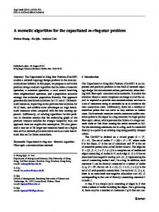
where β ∈ [0, 1] is a weighting coefficient which is fixed experimentally. Specifically, the subset SS is constructed as follows. At each iteration, a solution is randomly selected from population P and added into the subset SS if Eq.5 is satisfied. Whenever such a solution exists, this process is repeated until subset SS is filled with m solutions. Otherwise, we reconstruct the subset SS from scratch. 2.3.3. Multi-parent Recombination Operator Now we describe how our MPC operator works to generate new offspring solutions. Recall that the conventional OB crossover uses two phases to generate an offspring individual so from two parent individuals s1 and s2 . In the first phase, s1 is copied to so . In the second phase, OB selects k (here, k = n/2) positions and reorders the elements in these k selected positions according to their order in s2 . Readers are referred to [14] for details of the OB operator. Our MPC generalizes OB by employing m (m > 2) parent individuals to generate a new offspring solution. Given m selected parents {s1 , s2 , ..., sm }, the procedure of MPC also operates in two main phases. In the first phase, s1 is copied to so . In the second phase, we repeatedly choose k (k = n/m) different positions in so and rearrange the elements in these chosen positions according to their order in si (2 ≤ i ≤ m). Fig.1 shows an example of generating an offspring solution with OB and MPC. In this example, n = 6. In the example of OB, s1 is copied to so 8

OB Operator ‫ݏ‬ଵ ‫ݏ‬

ଶ

2 4

3 6

6 2

5 1

1 5

4 ‫ݏ‬௢

3

MPC Operator ‫ݏ‬ଵ

1

5

3

6

2

4

5

1

2

4

3

6

‫ݏ‬ଷ

4

3

1

6

2

5

‫ݏ‬ଶ

‫ݏ‬௢

2

4

6

5

1

3

The positions marked with circle are reordered elements from ‫ ݏ‬ଶ

1

5

3

6

4

2

The positions marked with circle are reordered elements from ‫ ݏ‬ଶ , the positions marked with square are reordered elements from ‫ ݏ‬ଷ

Figure 1: An example of MPC and OB first. Then we randomly choose positions (2, 4, 6) in so . The elements in these selected positions are (3, 5, 4) and these elements’ relative order in s2 is (4, 5, 3). So, we rearrange the selected elements according to their relative order in s2 . In the example of MPC, m = 3 and k = 2. We generate so in a similar way as OB. In the first step, s1 is copied to so . In the second step, we randomly choose positions (2,4) in so and rearrange the corresponding elements (5,6) according to their relative order in s2 , and then we randomly choose the positions (5,6) in so and rearrange the elements (2,4) according to their relative order in s3 . 2.4. Pool Updating In MPM, when c offspring individuals have been generated by the multiparent recombination operator, we immediately improve each of the offspring 9

individuals with the local search procedure. Then we update the population with these improved offspring individuals. For the purpose of maintaining a healthy population diversity [19, 20, 21], we devise a distance-and-quality based population updating strategy. The idea is that if an offspring solution is not good enough or too close to the individuals in the population, it should not be added to the population. In our updating strategy, we first create a temporary population of size p + c which is the union of the current population and the c offspring individuals. Then we calculate for each individual s a “score” by considering its quality and its distance to the other p + c − 1 individuals. Finally, we choose the p-best individuals to form the new population. The notion of score is defined as follows. Definition 1: (Distance between two solutions). Given two solutions sa = (a1 , a2 , ..., an ) and sb = (b1 , b2 , ..., bn ), we define the distance between sa and sb as n minus the length of their longest common subsequence (denoted by LCS). dis(sa , sb ) = n − LCS(sa , sb )

(6)

It is clear that a small value of dis(sa , sb ) indicates that the two solutions are similar to each other. The time complexity of calculating this distance is O(n2 ) [22]. Definition 2: (Distance between one solution and a population). Given a solution sa = (a1 , a2 , ..., an ) and a population P = {s1 , s2 , ..., sp }, the distance between sa and P is the minimum distance between sa and si (1 ≤ i ≤ p). dis(sa , P ) = min{dis(sa , si ), (1 ≤ i ≤ p), sa 6= si }

(7)

Definition 3: (Score of a solution with respect to a population). Given

10

a population P = {s1 , s2 , ..., sp }, the score of a solution si in P is defined as i e (si )) + (1 − α)A(dis(s e score(si , P ) = αA(f , P ))

(8)

e represents where f (si ) is the objective function value of solution si , and A() the normalized function:

e A(y) =

y − ymin ymax − ymin + 1

(9)

where ymax and ymin are respectively the maximum and minimum values of y in P . The number 1 is added to avoid 0 denominator. α is a parameter to balance the two parts of quality and distance. The score function is thus composed of two parts. The first part concerns the quality (objective function value) while the second part considers the diversity of the population. It is easy to check that if a solution has a high score, it is of good quality and is not too close to the other individuals in the population. Algorithm 2 describes the pseudo-code of our pool updating strategy.

11

Algorithm 2 Pseudo-code of population updating 1: INPUT: Population P = {s1 , ..., sp } and Offspring O = {o1 , ..., oc } 2: OUTPUT: Updated population P = {s1 , ..., sp } 3: P : P ′ ← P ∪ O /* Tentatively add all offspring O to population P */ 4: for i = 1, ..., p + c do

Calculate the distance between si and P according to Eq. 7

5:

6: end for 7: for i = 1, ..., p + c do

Calculate the score of each si in P according to Eq. 8

8:

9: end for 10: Sort the individuals in non-decreasing order of their scores 11: Choose the p best individuals to form P 12: return P

3. Computational Results and Comparisons In this section, we report experimental evaluations of our MPM algorithm by using the well-known LOLIB benchmark instances. We show computational results and compare them with the best known results obtained by the state-of-the-art algorithms in the literature. 3.1. Problem Instances and Experimental Protocol The LOLIB benchmarks have 484 instances in total and they are divided into 8 sets1 . The optimal solutions and best-known results for each instance can be found in [13]. IO: This is a well-known set of instances that contains 50 real-world linear ordering problems generated from input-output tables from various 1

All the instances are available at: http://www.optsicom.es/lolib/

12

sources. It was first used in [3]. SGB: These instances are from [23] and consist of input-output tables from sectors of the economy of the United States. The set has a total of 25 instances with 75 sectors. RandAI: There are 25 instances in each set with n = 100, 150, 200 and 500, respectively, giving a total of 100 instances. RandAII: There are 25 instances in each set with n = 100, 150 and 200, respectively, giving a total of 75 instances. RandB: 90 more random instances. MB: These instances have been used by Mitchell and Borchers for their computational experiments. xLOLIB: Some further benchmark instances have been created and used by Schiavinotto and St¨ utzle [10], giving a total of 78 instances. Special: 36 more instances used in [24, 25, 26]. Table 1: Sets of the tested instances Set IO SGB RandAI RandAII RandB MB xLOLIB Special Total

#Instances

#Optimal

#Lower Bound

50 25 100 75 90 30 78 36 484

50 25 25 70 30 29 229

100 50 20 78 7 255

Table 1 summarizes the number of instances in each instance class described above together with the information about the number of instances whose optimal solutions or lower bounds are known. Our MPM algorithm is programmed in C and compiled using GNU GCC on a PC running Windows XP with 2.4GHz CPU and 2.0Gb RAM. Given 13

the stochastic nature of the MPM, we solved each problem instance independently 50 times using different random seeds subject to a time limit of 2 hours. Note that the best known results listed in the following tables are also obtained within 2 hours, which are available at: http://www.optsicom.es/lolib/. 3.2. Parameter Setting Like all previous heuristic algorithms, MPM uses several parameters which are fixed via a preliminary experiments with a selection of problem instances. Precisely, we set p = 25, c = 10 and g = 30 (p is the population size, c is the offspring size and g means that if the average solution quality stays unchanged for g generations, the population is reconstructed). In the light of the experiments carried out in Section 4.1, we choose m = 3 to be the number of parents, β = rand(0.6, 0.7) for the parent selection and α = rand(0.8, 1.0) for the pool updating strategy. These settings are used to solve all the instances without any further fine-tuning of the parameters. 3.3. Computational Results We aim to evaluate the MPM’s performance on the LOLIB benchmark instances, by comparing its performance with the best-known results in the literature. Table 2 summarizes the computational statistics of our MPM algorithm on the instances with known optimal solutions. The name of each instance set is given in column 1, column 2 shows the number of instances for which the optimal results are obtained, column 3 gives the number of instances for which our algorithm matches the optimal solutions, column 4 presents the deviation from the optimal solutions and the average CPU time to match the optimal solutions is given in column 5.

14

Table 2: MPM’s performance on the instances with known optimal solutions Set IO SGB RandAII RandB MB Spec Total

#Optimal

#Match Optimal

#Dev(%)

Time(s)

50 25 25 70 30 29 229

50 25 25 70 30 29 229

0.0 0.0 0.0 0.0 0.0 0.0 0.0