Key words. parallel partition method, tridiagonal linear systems, parallel ... On a serial computer, Gaussian elimination without pivoting can be used to solve.
A MEMORY EFFICIENT PARALLEL TRIDIAGONAL SOLVER TRAVIS M. AUSTIN†, MARKUS BERNDT†, AND J. DAVID MOULTON† Abstract. We present a memory efficient parallel algorithm for the solution of tridiagonal linear systems of equations that are diagonally dominant on a very large number of processors. Our algorithm can be viewed as a parallel partitioning algorithm. We illustrate its performance using some examples. Based on this partitioning algorithm, we introduce a recursive version that has logarithmic communication complexity. Key words. parallel partition method, tridiagonal linear systems, parallel linear algebra AMS subject classifications. 15A06, 65F05, 65F50, 65Y05
1. Introduction. Large tridiagonal systems of linear equations appear in many numerical analysis applications. In our work, they arise in line relaxations needed by robust multigrid methods for structured grid problems [6, 7, 12]. Using this as our motivation, we present a new memory efficient partitioning algorithm for the solution of diagonally dominant tridiagonal linear systems of equations. This partitioning algorithm is well suited for distributed memory parallel computers. For simplicity, we assume in this paper that each processor has roughly the same number of subsequent rows of the tridiagonal system, and the number of processors NP is strictly less than the number of unknowns N . Note however that our algorithm can be applied to the case NP = N . On a serial computer, Gaussian elimination without pivoting can be used to solve a diagonally dominant tridiagonal system of linear equations in O(N ) steps. This algorithm, first described in [15], is commonly referred to as the Thomas algorithm. Unfortunately, this algorithm is not well suited for parallel computers. The first parallel algorithm for the solution of tridiagonal systems was developed by Hockney and Golub and described in 1965 in [9]. It is now usually referred to as cyclic reduction. Stone introduced his recursive doubling algorithm in 1973 [13]. Both cyclic reduction and recursive doubling are designed for fine grained parallelism, where each processor owns exactly one row of the tridiagonal matrix. In 1981, Wang proposed a partitioning algorithm that is aimed at more coarse-grained parallel computation, where NP 0.
(4.6)
7
A MEMORY EFFICIENT PARALLEL TRIDIAGONAL SOLVER (i−1)
(i−1)
Using diagonal dominance of vlk and vi , and vlk ,i−1 > 0, we show � � (i−1) (i−1) (i−1) (i−1) (i−1) vlk ,i−1 vi,i − vi,i−1 vlk ,i > |vlk ,jk | + |vlk ,i | (|vi,i−1 | + |vi,i+1 |) − vi,i−1 vlk ,i (i−1)
(i−1)
(i−1)
≥ |vlk ,jk ||vi,i−1 | + |vlk ,jk ||vi,i+1 | + |vlk ,i ||vi,i+1 | ≥ 0, (i)
which establishes (4.6). We now show diagonal dominance of vlk , which is equivalent to (i−1)
(i−1)
vlk ,i−1 vi,i − vi,i−1 vlk ,i
(i−1)
(i−1)
Using diagonal dominance of vi and vlk (i−1)
vi,i−1 vlk ,i
(i−1)
> |vlk ,jk vi,i−1 | + |vi,i+1 vlk ,i−1 |.
(4.7)
, we show
(i−1)
(i−1)
+ |vlk ,jk vi,i−1 | + |vi,i+1 vlk ,i−1 |
(i−1)
(i−1)
(i−1)
≤ |vi,i−1 vlk ,i | + |vlk ,jk vi,i−1 | + |vi,i+1 vlk ,i−1 | � � (i−1) (i−1) (i−1) = |vlk ,i | |vi,i−1 | + |vlk ,jk | + |vi,i+1 vlk ,i−1 | (i−1) (i−1)
(i−1)
< |vlk ,i vlk ,i−1 | + |vi,i+1 vlk ,i−1 | � � (i−1) (i−1) = |vlk ,i−1 | |vlk ,i | + |vi,i+1 | (i−1)
< vlk ,i−1 vi,i , which establishes (4.7). The proof for vuk is analogous. We remark that Theorem 4.1 implies that phase one of our algorithm is numeri(i) (i) cally stable, since at any time in the iterations vlk and vuk are diagonally dominant. Clearly, both phase two and three are stable, since the stable Thomas algorithm is used. In phase one of the algorithm, only six variables are needed to compute the interface equations on each processor. Note that the original tridiagonal system is not modified in this step. In the context of two-color zebra line relaxation in a multigrid method, the tridiagonal system does not need to be strored at all since the 2D matrix can be used directly to generate the interface equations. In contrast to Wangs’s partitioning algorithm, our algorithm does not require additional storage for a modified right hand side in phase one. In phase two, 4NP variables are needed on one of the processors to store one interface system, in addition to storing the coefficients of the complete interface tridiagonal system. In phase three of our algorithm, we need storage for one tridiagonal system, and we use the original right hand side. In the context of two-color zebra line relaxation, storage for one tridiagonal system of equations is enough. Since in phase three of our algorithm the original tridiagonal system is used, its coefficients can be taken directly from the 2D matrix. 5. Examples. In Figure 5.1, we show timings for 20 V (1, 1) cycles of symmetric BoxMG with alternating line relaxation. Here the problem size on the finest grid is fixed on all processors at 1000 × 1000. All timings are obtained on square processor grids, from 2×2 through 22×22 processors. The discrete problem was Poisson’s equation with the standard five-point stencil discretization. We observe a slight growth in the time per V-cycle in both the aggregate time as well as the time just for line
8
T. M. AUSTIN, M. BERNDT, J. D. MOULTON
16 total time for BoxMG aggregate time for line relaxation
14 12 seconds
10 8 6 4 2 0 0
100
200 300 number of processors
400
500
Fig. 5.1. Timings for 20 V (1, 1) BoxMG cycles with red-black line relaxation on square processor grids ranging from 2 × 2 to 22 × 22.
relaxation. Note that for the largest problem, lines span at most 22 processors. In the following, we consider lines that span significantly more processors. Denote by T (N, M, NP ) the time it takes to perform our line relaxation algorithm for a system of equations with N unknowns on NP processors for M lines. The scaled efficiency is then defined as E(N, M, P ) ≡ T (N, M, 1)/T (NP N, M, NP )
(5.1)
Figure 5.2 shows the scaled parallel efficiency of our line relaxation implementation for N = 1000 ∗ NP and M = 500. We see a slow degradation of scaled parallel efficiency to about 30% for NP = 250. Note that the interface problem is a tridiagonal system with 2 ∗ NP unknowns and that M of such interface problems must be solved. Since we gather all these equations on one of the processors and solve this interface system using the Thomas algorithm, our algorithm has a linear dependence on NP . However, we propose a recursive algorithm that is based on our partitioning algorithm: this algorithm reduces the dependency to a logarithmic dependence on P . Figure 5.3 shows detailed timings for the different phases of our algorithm. As expected, the calculation of the right hand side, phase 1, and phase 3 scale perfectly because no communication occurs. The complexity of phase 2 is linear in NP . In Figure 5.4, we show detailed timings for all parts of phase two of our algorithm. As expected, the complexity of each part of phase two appears to depend linearly on NP . The scatter operation has the strongest dependence on NP . In the next section, we propose a recursive version of our partitioning algorithm. This recursive partitioning algorithm will exhibit only logarithmic dependence on NP . 6. The recursive partitioning algorithm. For very large number of processors, the solution time for our parallel tridiagonal solver is dominated by the two communication steps in phase 2: scatter and gather. Our numerical experiments
9
A MEMORY EFFICIENT PARALLEL TRIDIAGONAL SOLVER
1 efficiency of line relaxation
parallel efficiency
0.8
0.6
0.4
0.2
0 50
100 150 number of processors
200
250
Fig. 5.2. Scaled linear efficiency on of the line relaxation for N = 1000NP and M = 500
25 aggegate time for line relaxation RHS calculation phase 1 phase 2 phase 3
seconds
20
15
10
5
0 50
100 150 number of processors
200
250
Fig. 5.3. Detailed timings for all parts of our partitioning algorithm for N = 1000NP and M = 500.
show that the scatter operation has a complexity of O(NP ), while the gather operation has a slightly better complexity. To alleviate this problem, we propose a recursive version of our partitioning algorithm. Since the interface system of equations is tridiagonal, diagonally dominant with positive diagonal entries, we solve using our partitioning algorithm. We do this by combining groups of interface equations on one processor. To be specific, we se-
10
T. M. AUSTIN, M. BERNDT, J. D. MOULTON
25 phase 2 gather scatter solve interface system
seconds
20
15
10
5
0 50
100 150 number of processors
200
250
Fig. 5.4. Detailed timings for all parts of phase two for N = 1000NP and M = 500.
lect MP groups of subsequent processors in such a way that there are roughly equal numbers of processors in each group. This can, for example, be accomplished by defining Mk ≡ bNP /MP c, k = 1, . . . , NP − 1 MMP ≡ NP − (MP − 1)bNP /MP c, Pk−1 Pk and assigning processors i=1 Mi +1 through i=1 Mk to group k, for k = 1, . . . , MP . After each processor has generated its two interface equations (phase one of our algorithm), these interface equations are gathered to the processor of lowest rank in the group. We call this processor the base processor in its group. This base processor now owns the part of the interface tridiagonal linear system that was generated in its group. If the number of groups is larger than Mk , we can proceed recursively by dividing the set of all base processors in several groups of roughly equal size Mk . Then each of the base processors generates two interface equations from its part of the interface tridiagonal linear system, and so forth After solving the interface system, the solution must be sent from the processor with lowest rank to all other processors in each group. This can be accomplished by using a scatter operation that involves all processors in each group. Since each processor is a member of only one group, all groups can perform these scatter operations simultaneously. Now we can proceed with phase three of our partitioning algorithm. Table 6.1 illustrates this coarsening procedure using 18 processors and a group size of at most three. Suppose that we are given a tridiagonal linear system of equations that is distributed across 18 processors (row A). Each processor runs through phase one of the non-recursive algorithm to generate two interface equations. Groups of three successive processors (row B) gather these interface equations to the lowest rank processor in their group (row C). In this example, now each of the lowest
11
A MEMORY EFFICIENT PARALLEL TRIDIAGONAL SOLVER
A B C D E F G
1 1 1 1 1 1 1
2 2
3 3
4 4 4 4
5 5
6 6
7 7 7 7
8 8
9 9
10 10 10 10 10 10
11 11
12 12
13 13 13 13
14 14
15 15
16 16 16 16
17 17
18 18
Table 6.1 Illustration of the coarsening procedure for 18 processors and a group size of three.
rank processors owns six equations of the first level interface tridiagonal system of equations. Processors 1, 4, 7, 10, 13, and 16 then each generate two new interface equations using their part of the first level interface tridiagonal system. Now the lowest rank processors are grouped in successive groups of three (row D) and gather the two interface equations that were just generated to the lowest rank processor in each group (row E) to form the second level interface tridiagonal system. Processors 1 and 10 make up just one group (row F) and each own a part of this second level interface tridiagonal system. Each of these two processors proceed to generate two interface equations from it, which are then gathered to processor 1, the lowest rank processor in this group, to form the third level interface tridiagonal system. This small linear system is solved directly (row F). The solution to the third level interface problem is now scattered to all processors in the group (row F) and used to compute the solution to the second level interface problem. The solution of the second level interface problem can now be computed (row E) and scattered to all processors in the level two groups (row D). This solution to the second level interface system is now used to compute the solution to the first level interface problem (row C), which is then scattered to all processors in the level one groups (row B). Now each processor knows the solution to the first level interface problem and can solve its part of the original problem. Since communication is orders of magnitude slower than computation, it is desirable to create groups with enough processors to balance communication and computation. The group size, for which the best performance is achieved, depends on the target computing architecture and must be determined experimentally for a given parallel computer. In the next section, we present a complexity analysis that can aid in determining the optimal group size. 7. Complexity analysis. Our numerical experiments indicate that the time for a scatter operation grows linearly with the number of participating processors. The gather operation also appears to scale linearly, albeit with a smaller slope. All three phases of our algorithm, without taking into account the communication, also scale linearly. Denote by L the number of lines that must be solved on a given set of processors to complete a sweep of line relaxation (e.g., the black lines) Denote by Nkmax = maxk=1,...,Np Nk the maximum number of equations that a single processor owns. Also, denote by γ, σ, and ρi , i = 1, 2, 3 the scaling factors of the gather operation, the scatter operation, and phase i, i = 1, 2, 3 of our algorithm, respectively. Then a simple model for the time it takes to complete our partitioning algorithm without recursion is T1 = (ρ1 + ρ3 )LNkmax + (γ + ρ2 + σ)LNp ,
(7.1)
12
T. M. AUSTIN, M. BERNDT, J. D. MOULTON
If we use one level of recursion, where we have MP groups and the maximum number of processors in a single group is Mkmax , then the complexity of the algorithm is T2 = (ρ1 + ρ3 )LNkmax + (γ + ρ1 + ρ3 + σ)LMkmax + (γ + ρ2 + σ)LMP
(7.2)
(`)
If we use multiple levels of recursion, where we have MP groups of processors on level ` and the maximum number of processors in a single group on level ` is Mk`max , then the complexity of the algorithm is T` = (ρ1 + ρ3 )LNkmax + (γ + ρ1 + ρ3 + σ)
` X
(`)
(`)
LMkmax + (γ + ρ2 + σ)LMP
(7.3)
i=2 (`)
Now assume a constant coarsening ratio, such that Mkmax is the same for all levels and the number of processors in each group is the same for all groups on all levels. We are interested in the case where the algorithm uses as many levels of recursion as possible, that number is `max = logMkmax NP . Then (7.3) becomes (`
)
T`max = (ρ1 + ρ3 )LNkmax + (γ + ρ1 + ρ3 + σ)(`max − 1)LMkmax + (γ + ρ2 + σ)LMP max . (7.4) Equation (7.4) suggests that the recursive algorithm should scale logarithmically with (` ) the number of processors. Note that MP max ≤ Mkmax is small and not dependent on NP . Note that the constants in (7.4) must be measured experimentally to determine the coarsening strategy for a given parallel computer. In the context of line relaxation in a multilevel scheme, the length of lines is halved on each coarser level. This will only affect the first term in (7.4), since Nkmax will be smaller on coarser multigrid levels. The other two terms in (7.4) do not depend on the length of a line. 8. Conclusions. We have introduced a new memory efficient partitioning algorithm for the solution of tridiagonal linear systems of equations. Based on this algorithm we proposed a recursive version of this algorithm that we expect to exhibit only logarithmic complexity with respect to the number of processors. This algorithm is different from other tridiagonal solvers with logarithmic complexity with respect to the number of processors, in that it can be tuned for a given parallel computer. We will explore this recursive algorithm in a forthcoming paper. REFERENCES [1] P. Amodio and L. Brugano, Parallel factorizations and parallel solvers for tridiagonal linearsystems, Linear Algebra and its Applications, 172 (1992), pp. 347 – 364. [2] P. Amodio, L. Brugano, and T. Politi, Parallel factorizations for tridiagonal matrices, SIAM J. Numer. Anal., 30 (1993), pp. 813 – 823. [3] T. M. Austin, M. Berndt, B. K. Bergen, J. E. Dendy, and J. D. Moulton, Parallel, scalable, and robust multigrid on structured grids, tech. report, Los Alamos National Laboratory, LA-UR-03-9167, 2003. [4] S. Bondeli, Divide and conquer: a parallel algorithm for the solution of a tridiagonal linear system of equations, Parallel Computing, 17 (1991), pp. 419–434. [5] P. N. Brown, R. D. Falgout, and J. E. Jones, Semicoarsening multigrid on distributed memory machines, SIAM J. Sci. Stat. Comput., 21 (2000), pp. 1823–1834. [6] J. E. Dendy, Black-box multigrid, Journal of Computational Physics, 48 (1982), pp. 366 – 386. [7] , Black-box multigrid for nonsymmetric problems, Applied Mathematics and Computation, 13 (1983), pp. 261 – 283.
A MEMORY EFFICIENT PARALLEL TRIDIAGONAL SOLVER
13
[8] J. E. Dendy, Two multigrid methods for three-dimensional problems with discontinuous and anisotropic coefficients., SIAM J. Sci. Stat. Comput., 8 (1987), pp. 673–685. [9] R. W. Hockney, A fast direct solution of poissons equation using fourier analysis, J. ACM, 12 (1965), pp. 95–113. [10] J. Hofhaus and E. F. V. de Velde, Alternating-direction line-relaxation methods on multicomputers, SIAM J. Sci. Comput., 17 (1996), pp. 454–478. [11] A. Povitzky, Parallelization of pipelined algorithms for sets of linear banded systems, J. Par. Distr. Comput., 59 (1999), pp. 68–97. [12] S. Schaffer, A semi-coarsening multigrid method for elliptic partial differential equations with highly discontinuous and anisotropic coefficients, SIAM J. Sci. Stat. Comput., 20 (1998), pp. 228–242. [13] H. S. Stone, An efficient parallel algorithm for the solution of a tridiagonal linear system of equations, J. ACM, 20 (1973), pp. 27–38. [14] X.-H. Sun, H. Z. Sun, and L. M. Ni, Parallel algorithms for solution of tridiagonal systems on multicomputers, in Proceedings of the 3rd international conference on Supercomputing, ACM Press New York, NY, USA, 1986, pp. 303–312. [15] L. H. Thomas, Elliptic problems in linear difference equations over a network, Watson Sci. Comput. Lab. Rept., Columbia University, New York, (1949). [16] C. H. Walshaw, Diagonal dominance in the parallel partition method for tridiagonal systems, SIAM J. Matrix Anal. Appl., 16 (1995), pp. 1086–1099. [17] H. H. Wang, A parallel method for tridiagonal equations, ACM Trans. Math. Software, 7 (1981), pp. 170–183. [18] P. Yalamov and V. Pavlov, On the stability of a partitioning algorithm for tridiagonal systems., SIAM Journal on Matrix Analysis and Applications, 20 (1998), pp. 159 – 81.