Jan 8, 2004 - in the baseband before digital-to-analog conversion, upcon- ..... Measured PA output PSD: (a) without predistortion; (b) with K = 5 memoryless ...
A MEMORY POLYNOMIAL PREDISTORTER IMPLEMENTED USING TMS320C67XX Lei Ding, Hua Qian, Ning Chen, G. Tong Zhou School of Electrical and Computer Engineering, Georgia Institute of Technology, Atlanta, GA 30332-0250, USA. ABSTRACT x(n)
z(n)
Up Predistortion D/A PA Digital baseband predistortion is a highly cost effective apConverter proach to linearize modern RF power amplifiers (PAs). TraPSfrag replacements ditionally, the PA is considered a memoryless nonlinear device. However, for wideband (such as WCDMA) and/or Down Predistorter A/D Converter Construction high power (such as base station) applications, PAs exhibit y(n)/G memory effects. Memory polynomial predistorter is shown to be a good choice for linearizing PAs with memory effects. In this paper, we investigate real-time implementaFig. 1. Predistortion System Diagram tion aspects of the memory polynomial predistorter. We implement the predistorter training algorithm on a Texas Instruments TMS320C67xx processor and evaluate the perconstructed as the pre-inverse of the nonlinear PA. Ideally, formance of the trained predistorter on our wideband digital the cascade of the two results in a linear gain to the origipredistortion testbed. nal input. With the predistorter, the PA can be utilized up to its saturation point while still maintaining good linearity, thereby significantly increasing its efficiency. To con1. INTRODUCTION struct the (adaptive) predistorter, a feedback path is often presented in the predistortion system. Recent transmission formats, such as wideband code division multiple access (WCDMA) and orthogonal frequency In the current literature, digital predistortion implemendivision multiplexing (OFDM), have high peak-to-average tations mostly focus on memoryless PAs (e.g. [2], [3], [4]); power ratios (PAPRs); i.e., large fluctuations in their signal i.e., the current output of the PA only depends on the curenvelopes. This characteristic makes these signals particurent input. However, as the signal bandwidth widens, PAs larly sensitive to the nonlinearity created by the RF power begin to exhibit memory effects, which may be due to the amplifier (PA) in the transmitter. Nonlinearity generates frequency-dependent behaviors of the components in the biout-of-band emission, also referred to as “spectral regrowth,” asing network or the thermal constants of the devices [5]. which interfere with adjacent channels. Nonlinearity also As a result, the PA becomes a nonlinear system with memcauses in-band distortion which degrades the bit error rate ory. To effectively linearize PAs with memory effects, preperformance. distorters also need to have memory structures. In [6],a One solution is to back off the PA so it operates within memory polynomial predistorter is shown to be robust against its linear region. However, for high PAPR signals, this reseveral types of nonlinear systems with memory. In this pasults in very low efficiency for the PA, typically less than per, we study real-time implementation aspects of the mem10% [1]; i.e., more than 90% of the dc power turns into heat ory polynomial predistortion system. and is thus wasted. Another solution is to allow the PA to operate in its nonlinear region to improve the efficiency and use techniques to linearize the PA. 2. MEMORY POLYNOMIAL MODEL Among all linearization techniques, digital predistortion is one of the most cost effective. It employs a predistorter Here, the predistorter adopts the model of Kim and Konin the baseband before digital-to-analog conversion, upconstantinou [7], version, and input to the PA (see Fig. 1). The predistorter is
This work supported in part by the National Science Foundation under Grant No. 0219262 and by the Texas Instruments DSP Leadership University Program.
z(n) =
Q K X X k=1 q=0
akq x(n − q)|x(n − q)|k−1 ,
(1)
which we call a memory polynomial. The input x(n), outx(n) put z(n) and coefficients akq of the model are all complex valued in general. Note that if the maximum delay Q = 0, (1) reduces to PSfrag replacements z(n) =
K X
Predistorter (Copy of A)
z(n)
FPGA/ASIC
=
q=0
=
Q X
x(n − q)
A/D
Down Converter
DSP
which is a conventional memoryless polynomial. A direct implementation of the predistorter model in (1) requires multiplications on the order of K 2 Q. However, an efficient implementation is possible by observing that (1) is equivalent to z(n)
y(n)/G
Predistorter Training (A)
(2)
k=1
Q X
PA
e(n)
zˆ(n)
ak0 x(n)|x(n)|k−1 ,
Up Converter
D/A
K X
akq |x(n − q)|
k−1
(3)
k=1
x(n − q) LUTq (|x(n − q)|),
(4)
q=0
[8], where the nonlinear polynomial for each delay q is implemented by a lookup table (LUT) indexed by |x(n − q)|. Therefore, only Q complex multiplications per sample are needed. 3. INDIRECT LEARNING ARCHITECTURE The indirect learning architecture [9] is used here to train the predistorter. This approach enables the predistorter to be constructed directly based on the input and output baseband data of the PA. Therefore, model assumption and parameter extraction of the PA are not necessary. Fig. 2 shows a block diagram of the predistorter training process. The feedback path labeled “Predistorter Training” (block A) has y(n)/G as its input, where G controls the intended gain of the linearized PA, and zˆ(n) as its output. Note that y(n) has been nominally matched with z(n); i.e., the relative delay and phase rotations have been taken care of. The actual predistorter is an exact copy of the feedback path (copy of A); it has x(n) as its input and z(n) as its output. Ideally, we would like y(n) = Gx(n), which renders z(n) = zˆ(n) and the error term e(n) = 0. Given y(n) and z(n), our task is to find the parameters of block A, which yields the predistorter. The algorithm converges when the error energy ||e(n)||2 is minimized. In Fig. 2, the predistorter performs the same computation, such as (4), for every input sample at high-speed. This kind of task is well suited for field programmable gate arrays (FPGAs) or application-specific integrated circuits (ASICs). The predistorter training block, however, involves relatively complex computations, which require a powerful digital signal processor (DSP), such as the Texas Instruments (TI) TMS320C67xx. The time required to train
Fig. 2. The indirect learning architecture for the predistorter. the predistorter determines the ability of the predistorter to response to changes in PA characteristics. Although these changes usually happen slowly, which may be due to temperature drift, aging, etc., a powerful DSP increases flexibility of the overall system. 4. PREDISTORTER CONSTRUCTION In the context of predistorter training (see the training block of Fig. 2), (1) becomes z(n) =
Q K X X
akq y(n − q)|y(n − q)|k−1 .
(5)
k=1 q=0
Since z(n) is linear in the parameters akq , the latter can be estimated by a simple least-squares method. By defining a new sequence rkq (n) = y(n − q)|y(n − q)|k−1 ,
(6)
we can rewrite (5) in matrix form as (7)
z = R a,
where z = [z(0), · · · , z(N − 1)]T , R = [R0 , · · · , RQ ], Rq = [r1q , · · · , rKq ], rkq = [rkq (0), · · · , rkq (N − 1)]T , and a = [a10 , · · · , aK0 , · · · , a1Q , · · · , aKQ ]T . The leastsquares solution for (7) is ˆ = (RH R)−1 RH z, a
(8)
where (·)H denotes complex conjugate transpose. The acˆ are directly related to curacy and stability of the solution a the numerical condition of the matrix RH R. A good indication of such condition is the condition number of the matrix [10, p. 258]; i.e., κ (RH R)
=
λmax , λmin
(9)
where λmax and λmin are, respectively, the largest and smallest eigenvalues of RH R. The matrix RH R generally has a
1. The nonlinear polynomials, such as y, y|y|, y|y|2 , etc., are highly correlated. 2. The data sample y(n) with different time indices are PSfrag replacements correlated. The correlation due to the first source can be greatly reduced by using the orthogonal polynomial proposed in [11]. In this formulation, (5) becomes z(n) =
Q K X X
bkq ψk (y(n − q)),
15
10
10
(a) (b) (c)
10
5
10
0
(d) 0
1
2
3
4
5
6
7
8
9
(10)
where k X
Ulk y |y|l−1
(11)
l=1
with Ulk =
10
Q
k=1 q=0
ψk (y) =
Condition Number
high condition number, which also means that there is large correlation between the columns of this matrix. There are two sources for this large correlation:
(−1)l+k (k + l)! . (l − 1)!(l + 1)!(k − l)!
(12)
For a K-th order polynomial, Ulk forms an upper triangular matrix U, which leads to the matrix form of (10), i.e., z = F b,
(13)
where F = [R0 U, · · · , RQ U]. The least-squares solution for b is then given by ˆ = (FH F)−1 FH z. b
Fig. 3. Condition number of the correlation matrix with different Q values and different input signals: (a) threecarrier WCDMA with K = 5 conventional polynomials; (b) three-carrier WCDMA with K = 5 orthogonal polynomials; (c) a complex random signal (amplitude uniformly distributed in [0,1]) with K = 5 conventional polynomials; (d) a complex random signal (amplitude uniformly distributed in [0,1]) with K = 5 orthogonal polynomials.
(14)
The orthogonal polynomial in [11] is derived for complex random signals with amplitude uniformly distributed between 0 and 1 (but is robust for non-uniformly distributed amplitudes as well). Therefore, to fully exploit the advantage of the orthogonal polynomial, the amplitude of y(n) should be scaled to the [0, 1] interval first before applying the ψk () operation. The correlation from the second source can be alleviated by using a special training signal whose samples at different time indices are independent. However, in many cases, dedicated training is not feasible. In this case, the accuracy ˆ can be improved by using higher precision of the solution a floating point numbers, such as using 64-bit double precision instead of 32-bit single precision. Fig. 3 shows an example of the condition number of the correlation matrix with different Q values and different input signals. We see that if the input signal is random with uniformly distributed amplitude in [0,1], the condition number is not affected by the number of delay terms, and
the orthogonal polynomial offers great advantages. For a three-carrier WCDMA signal, the benefit of using orthogonal polynomial decreases with the increase of the number of delay terms. However, a significant reduction of the condition number is still observed. 5. DSP IMPLEMENTATION Because of the benefits of orthogonal polynomials, we focused on DSP implementation using orthogonal polynomials. To evaluate the real-time performance of the predistorter training algorithm, we selected TI TMS320C6711, which is a low-cost yet powerful floating point processor. We implemented the algorithm in C and generated the DSPexecutable code with level-3 optimization provided by the TI C-compiler. 5.1. Implementation Details Figure 4 shows the flowchart of the algorithm. The algorithm starts with acquiring the baseband input and output data samples of the PA. The matrix R0 is then formed and multiplied with U to form the first K columns of F. The other columns of F are just shifted versions of the first K columns. Next, the upper triangular portion of the coefficients of the correlation matrix FH F are calculated. These coefficients are sufficient to define the whole matrix since the matrix is Hermitian. To obtain the solution for (14), we adopt the Cholesky decomposition approach, which is
very efficient in solving linear equations involving a Hermitian matrix [12]. Cholesky decomposition of FH F yields a lower-triangular matrix L such that L LH = FH F.
(15)
ˆ is the solution of Substituting (15) into (14), we see that b ˆ = FH z, L LH b
(16)
which can be obtained easily by using forward and back substitution [12, pp. 26-30]. 5.2. Performance Evaluation The computation requirement of the algorithm in the previous section is determined by two factors: the calculation of the correlation matrix and Cholesky decomposition. To give a quantitative measure of the complexity, we evaluate the floating point operations (flops) required by these two steps. For example, one complex multiplication involves six flops: four real multiplications, one real addition, and one real subtraction. It is straightforward to calculate the required number of flops once the C implementation is available. In our program, for a block of N data samples, the number of flops for obtaining FH F is approximately 4.5 K 2 (Q+1)2 N. The number of flops for obtaining the Cholesky decomposition is approximately 1.5 K 3 (Q + 1)3 . Therefore, when N is large, the computations are dominated by obtaining the correlation matrix. Table 1 shows the CPU cycles and execution time required by the C6711 starter kit to train the predistorter. We see that longer data lengths, more delay taps, and higher precision implementation all increase the computation time, although they all help to improve the predistortion performance. In practice, tradeoffs need to be made. The execution time shown here can be further reduced by (i) using new generations of TMS320C67xx processor, which are able to operate at a higher clock rate, (ii) coding the most time consuming block; i.e., the calculation of the correlation matrix, in assembly. 6. TESTBED MEASUREMENTS In this section, we present experimental results from our digital predistortion testbed, whose configuration is shown in Fig. 5. In the testbed, the digital I/O instrument is a Celerity system with 150 MSPS 16-bit digital input and output capability. It sends out 14-bit digital IF data streams to the DAC board continuously and acquires 12-bit digital IF data samples from the ADC when needed. The DAC and ADC used here are, respectively, AD9772 and AD9430 from Analog
Devices. The predistorter training algorithm is implemented on a TI C6711 starter kit, which connects with the Celerity system through a parallel port. A two-stage upconversion and downconversion chain were carefully assembled to avoid introducing extra distortions. In the experiment, the device under test (DUT) is a Siemens CGY0819 handset PA operating at the cellular band (824-849 MHz). The input to the PA is a 3.6 MHz bandwidth signal centered at 836 MHz. We tested both memoryless and memory polynomial predistorters on the PA. To evaluate the effects of the data length on predistortion performance, we trained each predistorter using 5,000 and 20,000 data samples. We used 64-bit implementation for both the memoryless and memory polynomial predistorters. The results are shown in Fig. 6 and Fig. 7. We see that the memory polynomial predistorter achieved more spectral regrowth suppression than the memoryless predistorter. This may be due to the memory effects in the PA or the frequency response caused by the analog filters in the upconverter. Moreover, training with a longer data length helped to improve the performance of the memory polynomial predistorter. Since the memory polynomial involves more parameters (K(Q + 1)) than the memoryless case (K), it is expected that the memory polynomial model needs more data points to estimate. 7. CONCLUSIONS In this paper, we investigated the real-time implementation aspects of the memory polynomial predistorter. While the actual predistorter is suitable for a FPGA or ASIC, the predistorter training algorithm requires a powerful DSP. Our predistorter training was based on orthogonal polynomials and Cholesky decomposition. We evaluated the computation requirements of this algorithm and tested it on a TI TMS320C6711 starter kit. The trained predistorters performed well on our experimental predistortion testbed. 8. REFERENCES [1] A. Wright and O. Nesper, “Multi-carrier WCDMA basestation design considerations - amplifier linearization and crest factor control,” PMC-Sierra, Santa Clara, CA, Technology White Paper, Aug. 2002. [2] P. B. Kenington, High-Linearity RF Amplifier Design. Boston, MA: Artech House, 2000. [3] J. K. Cavers, “Amplifier linearization using a digital predistorter with fast adaptation and low memory requirements,” IEEE Trans. Veh. Technol., vol. 39, no. 4, pp. 374–382, Nov. 1990.
[4] A. N. D’Andrea, V. Lottici, and R. Reggiannini, “RF power amplifier linearization through amplitude phase predistortion,” IEEE Transactions on communications, vol. 44, no. 11, pp. 1477–1484, November 1996. [5] J. H. K. Vuolevi, T. Rahkonen, and J. P. A. Manninen, “Measurement technique for characterizing memory effects in RF power amplifiers,” IEEE Trans. Microwave Theory Tech., vol. 49, no. 8, pp. 1383–1388, Aug. 2001. [6] L. Ding, G. T. Zhou, D. R. Morgan, Z. Ma, J. S. Kenney, J. Kim, and C. R. Giardina, “A robust predistorter constructed using memory polynomials,” IEEE Trans. Commun., Jan. 2004, to appear. [7] J. Kim and K. Konstantinou, “Digital predistortion of wideband signals based on power amplifier model with memory,” Electron. Lett., vol. 37, no. 23, pp. 1417–1418, Nov. 2001. [8] C. R. Giardina, J. Kim, and K. Konstantinou, “System and method for predistorting a signal using current and past signal samples,” U.S. Patent Application 09/915 042, July, 2001. [9] C. Eun and E. J. Powers, “A new Volterra predistorter based on the indirect learning architecture,” IEEE Trans. Signal Processing, vol. 45, no. 1, pp. 223–227, Jan. 1997. [10] T. K. Moon and W. C. Stirling, Mathematical Methods and Algorithms for Signal Processing. Englewood Cliffs, NJ: Prentice Hall, 1999. [11] R. Raich, H. Qian, and G. T. Zhou, “Digital baseband predistortion of nonlinear power amplifiers using orthogonal polynomials,” in Proc. IEEE Intl. Conf. Acoust., Speech, Signal Processing, Hong Kong, China, Apr. 2003, pp. 689–692.
PSfrag replacements
[12] D. S. Watkins, Fundamentals of Matrix Computations, 2nd ed. New York, NY: John Wiley & Sons, 2002.
START
Acquire PA input and output baseband data samples
Form F
Calculate FH F
Cholesky Decomposition of FH F
ˆ Obtain predistorter paramer b
Generate predistorter parameters and send it to FPGA/ASIC
Linearization Requirements Met?
Yes
No END
Fig. 4. Flow chart of the algorithm.
(a) K = 5, Q = 0
32-bit 64-bit
CPU Cycles 35094948 50879944
N=5000 Execution Time (s) 0.2351 0.3409
N= 20000 CPU Cycles Execution Time (s) 140036672 0.9382 203001588 1.3601
(b) K = 5, Q = 4
32-bit 64-bit
CPU Cycles 386017219 487638321
N=5000 Execution Time (s) 2.5863 3.2672
N= 20000 CPU Cycles Execution Time (s) 1542049416 10.3317 1969757008 13.1974
Table 1. Real-time performance of the predistorter training algorithm.
D/A
BPF1
Celerity Digital I/O System
BPF2
LO1
A/D
LPF6
BPF3
PreAmp
DUT
LO2
LPF5
BPF4
Atten
Load
TI C6711 Starter Kit
Fig. 5. Block diagram of the testbed.
20:31:48 Jan 8, 2004 Ref -20 dBm Samp Log 8 dB/
Trace/View Mkr1 ∆ 2.37 MHz -45.76 dB
Atten 5 dB
*
Trace 1
2
3
1R
Clear Write
Max Hold
VAvg 100 V1 V2 V3 FC AA
Min Hold
(a) (b)
View
1
(c) Blank
Center 836 MHz #Res BW 30 kHz
VBW 30 kHz
More
Span 12 MHz Sweep 27.16 ms (401 pts)
1 of 2
Fig. 6. Measured PA output PSD: (a) without predistortion; (b) with K = 5 memoryless predistorter trained by 5,000 data samples; (c) with K = 5 memoryless predistorter trained by 20,000 data samples. (b) and (c) coincide.
20:28:27 Jan 8, 2004 Ref -20 dBm Samp Log 8 dB/
Trace/View Mkr1 ∆ 2.37 MHz -48.49 dB
Atten 5 dB
*
Trace 1
2
3
1R
Clear Write
Max Hold
Min Hold
VAvg 100 V1 V2 V3 FC AA
(a) (b) 1
View
(c) Blank
Center 836 MHz #Res BW 30 kHz
VBW 30 kHz
Span 12 MHz Sweep 27.16 ms (401 pts)
More 1 of 2
C:\STATE055.STA file saved
Fig. 7. Measured PA output PSD: (a) without predistortion; (b) with K = 5, Q = 4 memory polynomial predistorter trained by 5,000 data samples; (c) with K = 5, Q = 4 memory polynomial predistorter trained by 20,000 data samples.