POLYNOMIAL PRESERVING GRADIENT ... - Semantic Scholar

c 2004 Institute for Scientific ° Computing and Information

INTERNATIONAL JOURNAL OF NUMERICAL ANALYSIS AND MODELING Volume 1, Number 1, Pages 1–24

POLYNOMIAL PRESERVING GRADIENT RECOVERY AND A POSTERIORI ESTIMATE FOR BILINEAR ELEMENT ON IRREGULAR QUADRILATERALS ZHIMIN ZHANG Abstract. A polynomial preserving gradient recovery method is proposed and analyzed for bilinear element under quadrilateral meshes. It has been proven that the recovered gradient converges at a rate O(h1+ρ ) for ρ = min(α, 1), when the mesh is distorted O(h1+α ) (α > 0) from a regular one. Consequently, the a posteriori error estimator based on the recovered gradient is asymptotically exact. Key Words. Finite element method, quadrilateral mesh, gradient recovery, superconvergence, a posteriori error estimate.

1. Introduction A posteriori error estimation is an active research area and many methods have been developed. Roughly speaking, there are residual type error estimators and recovery type estimators. For the literature, readers are referred to recent books by Ainsworth-Oden [2] and by Babuˇska-Strouboulis [4], a conference proceeding [16], a survey article by Bank [5], an earlier book by Verf¨ urth [23], and references therein. While residual type estimators have been analyzed extensively, there is only limited theoretical research on recovery type error estimators (see, e.g., [2, Chapter 4], [6, 7, 9, 10, 15, 22, 28, 29]). Yet, recovery type error estimators are widely used in engineering applications and their practical effectiveness has been recognized by more and more researchers. Currently, ZZ patch recovery is used in commercial codes, such as ANSYS, MCS/NASTRANMarc, Pro/MECHANICA (a product of Parametric Technology), and IDEAS (a product of SDRC, part of EDS), for the purpose of smoothing and adaptive re-meshing. It is also used in NASA’s COMET-AR (COmputational MEchanics Testbed With Adaptive Refinement). In a computer based investigation [4] by Babuˇska et al., it was found that among all error estimators tested (including the equilibrated residual error estimator, the ZZ patch recovery error estimator, and many others), the ZZ patch recovery error estimator based on the discrete least-squares fitting is the most robust. Received by the editors December 17, 2003. 2000 Mathematics Subject Classification. 65N30, 65N15, 41A10, 41A25, 41A27, 41A63. This research was partially supported by the National Science Foundation grants DMS-0074301 and DMS-0311807. 1

2

ZHIMIN ZHANG

It is worth pointing out that the recovery type error estimator was originally based on finite element superconvergence theory, in hopes that a recovered gradient was superconvergent and hence could be used as a substitute of the exact gradient to measure the error. The reader is referred to [4, 11, 16, 18, 25, 33] for literature regarding superconvergence theory. In order to prove superconvergence, it is necessary to impose some strong restrictions on mesh, which are usually not satisfied in practice. Nevertheless, it is found that in many practical situations, recovery type error estimators perform astonishingly well under meshes produced by the Delaunay triangulation. Mathematically, this fact has not yet been rigorously justified. In a recent work, Bank-Xu [6, 7] introduced a recovery type error estimator based on global L2 -projection with smoothing iteration of the multigrid method, and they established asymptotic exactness in the H 1 -norm for linear element under shape regular triangulation. However, the recovery operator is a global one. On the other hand, Wang proposed a “semi-local” recovery [27] and proved its superconvergence under the quasi-uniform mesh assumption. The main feature of his method is to apply L2 projection on a coarser mesh with size τ = Chα with α ∈ (0, 1). Consequently, there is no upper bound for the number of elements in an element patch when mesh size h → 0. As for element-wise recovery operators, Schatz-Wahlbin et al. [15, 22] established a general framework which requests, for linear element, given a fixed 0 < ² < 1, that ! Ãµ ¶ µ ¶² H 2 ² h H < 1. m=C h + ln h H h Here h is the size of element τ , H ≥ 2h is the size of the patch ωτ (surrounding τ ), where the recovery takes place, and C is an unknown constant which comes from the analysis. Let H = Lh. In order for m < 1, we need C(L2 h² + L−² ln L) < 1. Depending on C, this essentially asks for sufficiently large L and sufficiently small h, which implies many elements may be needed for the recovery operator. Nevertheless, in practice, many recovery operators work well with an H/h that is not large (usually 2). Therefore a theoretical justification for recovery that involves only a few elements surrounding a node is necessary. In other word, it is desired to study the case when H = 2h. The situation is further complicated by quadrilateral meshes where mappings between the reference element and physical elements are not affine. We encounter some delicate theoretical issue in analysis. See [1, 3, 8, 13, 14, 19, 21, 30, 31, 36] for more details. In this article, we propose and analyze a gradient recovery method which is different from the ZZ recovery [34]. We show that the a posteriori estimate based on this new recovery operator is asymptotically exact under mesh distortion O(h1+α ) when α > 0. Here α = ∞ represents the uniform mesh and α = 0 represents completely unstructured mesh. The main feature of this new recovery operator is:

POLYNOMIAL PRESERVING GRADIENT RECOVERY

3

(1) It is completely local just like the ZZ patch recovery; (2) It is polynomial preserving under practical meshes, a property not shared by the ZZ; (3) It is superconvergent under minorly restricted mesh conditions; (4) It results in an asymptotically exact error estimator when the mesh is not overly distorted. The error bound is in the form of (1.1)

ηh + O(h1+ρ ) ≤ k∇(u − uh )k ≤ ηh + O(h1+ρ ),

rather than 1 ηh + higher order term ≤ k∇(u − uh )k ≤ Cηh + higher order term C in most error bounds in the literature. Here C is an unknown constant, which may be very large and hence makes the error bound not very meaningful in practice. We comment that hα can be reduced to o(1) and still maintain the asymptotic exactness of the error estimator. If we give up the asymptotic exactness requirement and only ask for a reasonable error estimator, we may further reduce the condition to “a sufficiently small constant γ > 0”. The main results of this paper include a super-close property (Theorem 3.3), a global superconvergent recovery result (Theorem 4.2), and a local superconvergent recovery result (Theorem 4.3). The error bound (1.1) is a consequence of Theorems 4.2 or 4.3. All these results need a mesh assumption, Condition (α), which is introduced in Section 2. Basically, we allow quadrilaterals to be asymptotically distorted by O(h1+α ) (α > 0) from parallelograms. Note that α = 0 represents arbitrary meshes. Therefore, the mesh considered here is next to arbitrary (with a little structure). Indeed, when a very practical mesh refinement strategy, bisection (link edge-center of each opposite side of a quadrilateral) is applied, we have α = 1 (see Lemma 2.1). 2. Geometry of the Quadrilateral ˆ = [−1, 1]×[−1, 1] be the reference element with vertices Zî , and let Let K K K be a convex quadrilateral with vertices ZiK (xK i , yi ), i = 1, 2, 3, 4. There ˆ = K, FK (Zî ) = Z K exists a unique bilinear mapping FK such that FK (K) i given by 4 4 X X xK N , y = yiK Ni , x= i i i=1

where

1 N1 = (1 − ξ)(1 − η), 4 1 N3 = (1 + ξ)(1 + η), 4 We can also express x = a0 + a1 ξ + a2 η + a3 ξη,

i=1

1 N2 = (1 + ξ)(1 − η), 4 1 N4 = (1 − ξ)(1 + η). 4 y = b0 + b1 ξ + b2 η + b3 ξη;

4

ZHIMIN ZHANG

where by suppressing the index “K”, 4a0 = x1 + x2 + x3 + x4 , 4a1 = −x1 + x2 + x3 − x4 , 4a2 = −x1 − x2 + x3 + x4 , 4a3 = x1 − x2 + x3 − x4 ,

4b0 4b1 4b2 4b3

= y1 + y2 + y3 + y4 ; = −y1 + y2 + y3 − y4 ; = −y1 − y2 + y3 + y4 ; = y1 − y2 + y3 − y4 .

To any function v(x, y) defined on K, we associate vˆ(ξ, η) by vˆ(ξ, η) = v(x(ξ, η), y(ξ, η)),

or vˆ = v ◦ FK .

The Jacobi matrix of the mapping FK is µ ¶ µ ¶ xξ yξ a1 + a3 η b1 + b3 η (DFK )(ξ, η) = = . xη yη a2 + a3 ξ b2 + b3 ξ Let ∇v = (∂x v, ∂y v)T , it is straight forward to verify that (2.1)

ˆ v = (∂ξ vˆ, ∂η vˆ)T = DFK ∇v, ∇ˆ

(2.2)

∂ξrr vˆ = [(a1 + a3 η)∂x + (b1 + b3 η)∂y ]r v,

(2.3)

∂ξr+1 ˆ = r[(a1 + a3 η)∂x + (b1 + b3 η)∂y ]r−1 (a3 , b3 ) · ∇v rη v +[(a1 + a3 η)∂x + (b1 + b3 η)∂y ]r [(a2 + a3 ξ)∂x + (b2 + b3 ξ)∂y ]v,

r+1 and ∂ηrr vˆ and ∂ξη ˆ can be expressed in a similar way. The determinant of r v the Jacobi matrix is

JK = JK (ξ, η) = J0K + J1K ξ + J2K η, where J0K = a1 b2 − b1 a2 ,

J1K = a1 b3 − b1 a3 ,

J2K = b2 a3 − a2 b3 .

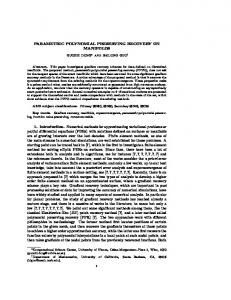
The inverse of the Jacobi matrix is ¶ µ µ ¶ 1 ξx ηx b2 + b3 ξ −b1 − b3 η −1 = (DFK ) = . ξy ηy JK −a2 − a3 ξ a1 + a3 η Note that a3 = b3 = 0 when K is a parallelogram in which case FK is an affine mapping, and further a3 = b3 = a2 = b1 = 0 when K is a rectangle. Starting from Z1 , we express the four edges (with the midpoint Pi ) as four vectors v i , i = 1, 2, 3, 4, pointing counter-clock-wisely (Figure 1). We denote the midpoints of Z2 Z4 and Z1 Z3 as O1 and O2 , respectively. For analysis purpose, it is convenient to identify 2-D vectors as 3-D vectors by adding the third component 0. We can verify that 1 P4 P2 = (x2 + x3 − x4 − x1 , y2 + y3 − y4 − y1 , 0) = 2(a1 , b1 , 0), 2 1 P1 P3 = (x3 + x4 − x1 − x2 , y3 + y4 − y1 − y2 , 0) = 2(a2 , b2 , 0), 2 1 O1 O2 = (x1 + x3 − x2 − x4 , y1 + y3 − y2 − y4 , 0) = 2(a3 , b3 , 0). 2 Then q q q (2.4) 2 a21 + b21 = |P4 P2 |, 2 a22 + b22 = |P1 P3 |, 2 a23 + b23 = |O1 O2 |.


5

5 Z3

4 P3 Z4

3

v2

v3

2

o2

1

o1

θ2

P

2

O

0

2

O

P4

−1

O

1

θ1

−2 −3 v

4

−4 −5 −6

v1

P1

Z1 −4

−2

0

2

4

Z2

6

Figure 1. Geometry of a quadrilateral (2.5) (2.6) (2.7)

4(a1 a2 + b1 b2 ) = P4 P2 · P1 P3 = |P4 P2 ||P1 P3 | cos αK , 4(a1 a3 + b1 b3 ) = P4 P2 · O1 O2 = |P4 P2 ||O1 O2 | cos βK , 4(a2 a3 + b2 b3 ) = O1 O2 · P1 P3 = |O1 O2 ||P1 P3 | cos γK ,

where the meaning of angles αK , βK , and γK is obvious from the context. ¯ ¯ ¯ i j k¯ ¯ ¯ 1 1 (2.8) J0K k = ¯¯a1 b1 0¯¯ = P4 P2 × P1 P3 = |P4 P2 ||P1 P3 | sin αK , 4 4 ¯a2 b2 0¯ ¯ ¯ ¯ i j k¯ ¯ ¯ 1 1 (2.9) J1K k = ¯¯a1 b1 0¯¯ = P4 P2 × O1 O2 = |P4 P2 ||O1 O2 | sin βK , 4 4 ¯a3 b3 0¯ ¯ ¯ ¯ i j k¯ ¯ ¯ 1 1 (2.10) J2K k = ¯¯a2 b2 0¯¯ = P1 P3 × O1 O2 = |P1 P3 ||O1 O2 | sin γK . 4 4 ¯a3 b3 0¯ We could also express |J1K | = 2|(x4 −x3 )(y2 −y1 )−(x2 −x1 )(y4 −y3 )| = 2|vv 3 ×vv 1 |,

|J2K | = 2|vv 4 ×vv 2 |.

Let hK be the longest edge length of K, we introduce the following condition: Definition 1. A convex quadrilateral K is said to satisfy the diagonal condition if (2.11)

dK = |O1 O2 | = O(h1+α K ),

α ≥ 0.

Note that K is a parallelogram if and only if dK = 0. Therefore, the distance between the two diagonal mid-points O1 and O2 is a convenient measure for the deviation of a quadrilateral from a parallelogram. The two extremal

6

ZHIMIN ZHANG

cases α → ∞ and α → 0 represent parallelogram and completely unstructured quadrilateral, respectively. Anything in between will pose some restriction, especially α = 1 is the well-known 2-strongly regular partition, see, e.g., [13, 36]. The diagonal condition was previously used by Chen [12] for triangular meshes, where two adjacent triangles form a quadrilateral that satisfies the condition. The following lemma states a known fact regarding the 2-strongly regular partition (α = 1). Although this fact is widely used, we have not seen a formal proof of it in the literature. An elementary proof is therefore provided in the Appendix. Lemma 2.1. Let o1 o2 be the distance between two diagonal mid-points of any of four refined quadrilaterals through the bi-section of K. Then 1 |o1 o2 | = |O1 O2 |. 4 Recall that the bi-section reduces the length of longest edge by half, which is hK /2. Therefore, the diagonal condition (2.11) is satisfied with α = 1. To measure this deviation, Rannarchar and Turek [21] used the quantity σK = max(|π − θ1 |, |π − θ2 |), where θ1 and θ2 are the angles between the outward normals of two opposite sides of K. Definition 2. A convex quadrilateral K is said to satisfy the angle condition if (2.12)

σK = O(hαK ),

α ≥ 0.

Lemma 2.2. The diagonal condition (2.11) and the angle condition (2.12) are equivalent in the sense α dK = O(h1+α K ) ⇐⇒ σK = O(hK ),

α ≥ 0.

A special case of this lemma has been proved in [19, Theorem 4.13] under some complicated mesh restrictions. Here we provide a direct and much simpler proof in the Appendix without any mesh assumption. Definition 3. A partition Th is said to satisfy Condition (α) if there exist α > 0 such that i) Any K ∈ Th satisfies the diagonal condition (2.11). ii) Any two K1 , K2 in Th that share a common edge satisfy a neighboring condition: For j = 1, 2, (2.13)

K2 α α 1 aK j = aj (1 + O(hK1 + hK2 )),

K2 α α 1 bK j = bj (1 + O(hK1 + hK2 )).

To assure optimal order error estimates in the H 1 -norm for the bilinear isoparametric interpolation on a convex quadrilateral K, namely, the estimate (2.14)

ku − uI k0,K + h|u − uI |1,K ≤ Ch2K |u|2,K ,


7

we need a degeneration condition, which was introduced by Acosta and Durán [1]. Definition 4. A convex quadrilateral K is said to satisfy the Regular decomposition property with constants N ∈ R and 0 < Ψ < π, or shortly RDP (N, Ψ), if we can divide K into two triangles along one of its diagonals, which will always be called d1 , in such a way that |d1 |/|d2 | ≤ N and both triangles satisfy the maximum angle condition with parameter Ψ (i.e., all angles are bounded by Ψ). Remark. This is a weaker condition than many other similar degenerate conditions, cf. e.g., [13, 14, 31, 36]. It was proved in [1] that RDP (N, Ψ) is a sufficient condition for (2.14) to be hold, and the authors conjectured that it is also a necessary condition. Recently, Ming-Shi confirmed this conjecture by a simple counter-example [19]. We denote X = X(ξ, η) = X0 + X1 where ¶ ¶ µ µ b2 −b1 b3 X0 = , X1 = X1 (ξ, η) = (ξ, −η). −a2 a1 −a3 Lemma 2.3. Let a convex quadrilateral K satisfy the diagonal condition. Then kX0 X −1 k2 = 1 + O(hαK ),

kX1 X −1 k2 = kI − X0 X −1 k2 = O(hαK ).

Proof: It is straightforward to verify that ¶ µ ¶ ¸ ¶ ·µ µ η a1 b1 b2 −b1 1 −1 + (a3 , b3 ) X0 X = ξ a2 b2 −a2 a1 JK ¶µ ¶ µ J0K 1 η b2 −b1 = (a3 , b3 ) I+ ξ −a a JK JK 2 1 where I is a 2-by-2 identity matrix; and X1 X

−1

= I − X0 X

−1

JK JK 1 = ( 1 ξ + 2 η)I − JK JK JK

µ

b2 −b1 −a2 a1

¶µ ¶ η (a3 , b3 ). ξ

By the definition of JK and geometric relations of (2.4), (2.8)–(2.10), we see that J0K J1K J2K = 1 + O(hαK ), = O(hαK ), = O(hαK ), JK JK JK by the diagonal condition (2.11). The desired conclusion follows. 2 3. Superconvergence Analysis We consider the variational problem: Find u ∈ H 1 (Ω) such that (3.1) a(u, v) = (∇u, A∇v) + (bb · ∇u, v) + (cu, v) = (f, v),

∀v ∈ H 1 (Ω),

where A is a 2-by-2 symmetric positive definite matrix and Ω is a polygonal domain which allows a quadrilateral partition Th with h = max hK . We K∈Th

assume that all functions are sufficiently smooth, in particular, (3.2)

kA − A0 k0,∞,K = O(hαK ),

kbb − b 0 k0,∞,K = O(hαK ),

8

ZHIMIN ZHANG

where A0 and b 0 are piece-wisely constant functions that on each K ∈ Th , Z Z 1 1 A0 |K = A(x, y)dxdy, b 0 |K = b (x, y)dxdy. |K| K |K| K We also assume that a(·, ·) satisfies the inf-sup condition to insure that (3.1) has a unique solution. Using 1 ˆ v, ∇v = X ∇ˆ JK we write Z Z 1 ˆ w) ˆ ∇ˆ ˆ v )dξdη, (∇w, A∇v)K = (∇w)T A∇vdxdy = (X ∇ ˆ T A(X J ˆ K K K Z Z ˆ wdξdη; (bb · ∇w, v)K = vbb · ∇wdxdy = vˆbˆ · X ∇ ˆ ˆ K

K

and define (∇w, A∇v)∗K

(3.3)

Z 1 ˆ w) ˆ v )dξdη = (X0 ∇ ˆ T A0 (X0 ∇ˆ J0K Kˆ Z ˆ w) ˆ v dξdη, = (∇ ˆ T B K ∇ˆ ˆ K

Z (bb · ∇w, v)∗K = b 0 · X0

(3.4)

ˆ K

ˆ wdξdη, vˆ∇ ˆ

where

1 K (X K )T AK 0 X0 . J0K 0 We introduce the following lemma, which can be verified by straightforward calculation. BK =

Lemma 3.1. Under the condition (2.13) and (3.2), we have J0K1 = J0K2 (1 + O(hαK1 + hαK2 )),

kB K1 − B K2 k = O(hαK1 + hαK2 ).

Theorem 3.1. Let the assumption (3.2) be satisfied, and let K satisfy the diagonal condition. Then there exists a constant C independent of u and K, such that (3.5)

|(∇w, A∇v)K − (∇w, A∇v)∗K | ≤ ChαK k∇wk0,K k∇vk0,K ,

(3.6)

|(bb · ∇w, v)K − (bb · ∇w, v)∗K | ≤ ChαK k∇wk0,K kvk0,K .

Proof: We decompose (3.7)

(∇w, A∇v)K − (∇w, A∇v)∗K = (∇w, (A − A0 )∇v)K Z 1 ˆ w) ˆ v ) − (X0 ∇ ˆ w) ˆ v )]dξdη + [(X ∇ ˆ T A0 (X ∇ˆ ˆ T A0 (X0 ∇ˆ J ˆ K ZK 1 1 ˆ w) ˆ v )dξdη. ˆ T A0 (X0 ∇ˆ + ( − K )(X0 ∇ J ˆ J K K 0

By (3.2) (3.8)

|(∇w, (A − A0 )∇v)K | ≤ ChαK k∇wk0,K k∇vk0,K .


9

Using X = X0 + X1 , we express Z 1 ˆ w) ˆ v ) − (X0 ∇ ˆ w) ˆ v )]dξdη [(X ∇ ˆ T A0 (X ∇ˆ ˆ T A0 (X0 ∇ˆ ˆ JK K Z 1 ˆ w) ˆ v ) + (X1 ∇ ˆ w) ˆ v) = [(X0 ∇ ˆ T A0 (X1 ∇ˆ ˆ T A0 (X0 ∇ˆ J ˆ K K ˆ w) ˆ v )]dξdη. + (X1 ∇ ˆ T A0 (X1 ∇ˆ The first term can be estimated as Z 1 ˆ w) ˆ v )dξdη| | (X0 ∇ ˆ T A0 (X1 ∇ˆ J ˆ K K Z 1 1 ˆ w) ˆ v )JK dξdη| = | ( X∇ ˆ T X −T X0T A0 X1 X −1 ( X ∇ˆ J J ˆ K K K Z = | (∇w)T (X0 X −1 )T A0 X1 X −1 ∇vdxdy| K

≤ ChαK k∇wk0,K k∇vk0,K . Note that (X0 X −1 )T A0 X1 X −1 = O(hαK ) by Lemma 2.3. The other two terms can be estimated similarly. Then we derive Z 1 ˆ w) ˆ v ) − (X0 ∇ ˆ w) ˆ v )]dξdη| (3.9) [(X ∇ ˆ T A0 (X ∇ˆ ˆ T A0 (X0 ∇ˆ | J ˆ K K ≤ ChαK k∇wk0,K k∇vk0,K . Next Z

1 1 ˆ w) ˆ v )dξdη| − K )(X0 ∇ ˆ T A0 (X0 ∇ˆ ˆ JK J0 K Z JK 1 1 ˆ w) ˆ v )JK dξdη| = | (1 − K )( X∇ ˆ T X −T X0T A0 X0 X −1 ( X ∇ˆ JK ˆ J0 JK K Z JK JK = | (− 1K ξ(x, y) − 2K η(x, y))(∇w)T (X0 X −1 )T A0 X0 X −1 ∇vdxdy| J0 J0 K α ≤ ChK k∇wk0,K k∇vk0,K .

(3.10) |

(

Note that by Lemma 2.3, J1K J2K ξ(x, y) + η(x, y) = O(hαK ), J0K J0K

(X0 X −1 )T A0 X0 X −1 = 1 + O(hαK ).

We then obtain (3.5) by applying (3.8)-(3.10) to the right hand side of (3.7). Now we write the convection term as following: (3.11)

(bb · ∇w, v)K − (bb · ∇w, v)∗K Z Z ˆ ˆ ˆ wdξdη. = vˆb · (X − X0 )∇wdξdη ˆ + vˆ(bˆ − b 0 ) · X0 ∇ ˆ ˆ K

ˆ K

10

ZHIMIN ZHANG

We estimate the two terms separately. Z ˆ wdξdη| (3.12) | vˆbˆ · (X − X0 )∇ ˆ ˆ K Z ˆ wdξdη| = | vˆˆb · (I − X0 X −1 )X ∇ ˆ ˆ K Z = | vbb · (I − X0 X −1 )∇wdxdy| K

≤ ChαK k∇wk0,K kvk0,K , by Lemma 2.3. (3.13)

Z |

ˆ K

ˆ wdξdη| vˆ(ˆb − b0 ) · X0 ∇ ˆ

Z = |

ˆ K

ˆ w)dξdη| vˆ(bˆ − b 0 ) · X0 X −1 (X ∇ ˆ

Z = |

K

v(bb − b 0 ) · X0 X −1 ∇wdxdy|

≤ ChαK k∇wk0,K kvk0,K , by Lemma 2.3 and (3.2). Applying (3.12) and (3.13) to (3.11), we obtain (3.6). 2 We then define two modified bilinear forms X X ah (u, v) = ah (u, v)K , bh (w, v) = bh (u, v)K K

K

where (3.14)

ah (u, v)K = (∇u, A∇v)∗K + (bb · ∇u, v)K + (cu, v)K ,

(3.15)

bh (u, v)K = (∇u, A∇v)∗K + (bb · ∇w, v)∗K + (cu, v)K .

Given a quadrilateral partition Th on a polygonal domain Ω, we define the bilinear finite element space ˆ ∀K ∈ Th }. Sh = {v ∈ H 1 (Ω) : vˆ = v ◦ FK ∈ Q1 (K), Theorem 3.2. Let Th satisfy the condition (α) and RDP (N, Ψ), and let uI ∈ Sh be the bilinear interpolation of u ∈ H 3 (Ω) ∩ H01 (Ω). Then there exists a constant C independent of h and u, such that for any v ∈ Sh , |ah (u − uI , v)| + |bh (u − uI , v)| ≤ C(h1+α |u|2,Ω + h2 |u|3,Ω )kvk1,Ω . Proof: For convenience, we set w = u − uI . By (3.14) and (3.15), we can express X ah (w, v) − bh (w, v) = [(bb · ∇w, v)K − (bb · ∇w, v)∗K ]. K∈Th

Recall (3.6), and we have (3.16)

|ah (w, v) − bh (w, v)| ≤ C

X

hαK k∇wk0,K kvk0,K

K∈Th 1+α

≤ Ch

|u|2,Ω kvk0,Ω ,


11

since by the RDP (N, Ψ) assumption, (2.14) is valid. Therefore, we only need to estimate bh (w, v). Again, by the RDP (N, Ψ) assumption, we have |(cw, v)| ≤ Ch2 |u|2,Ω kvk0,Ω .

(3.17)

Hence, our task is narrowed down to estimate (∇u, A∇v)∗K ,

and (bb · ∇w, v)∗K

for K ∈ Th . By the definition (3.3) and (3.4), we see that all coefficients are constants now and we only need to estimate following terms Z Z Z Z Z Z ∂ξ w∂ ˆ ξ vˆ, ∂ξ w∂ ˆ η vˆ, ∂η w∂ ˆ ξ vˆ, ∂η w∂ ˆ η vˆ, vˆ∂ξ w, ˆ vˆ∂η w. ˆ ˆ K

ˆ K

ˆ K

ˆ K

ˆ K

ˆ K

ˆ There are only two terms ξ 2 , η 2 not in the reference a) Let u ˆ ∈ P2 (K). space of the bilinear interpolation, therefore, Z ∂ξ w∂ ˆ ξ vˆ = 0, ∀v ∈ Sh . ˆ K

By the Bramble-Hilbert Lemma, Z (3.18) | ∂ξ w∂ ˆ ξ vˆ| ≤ CkD3 u ˆkL2 (K) ˆkL2 (K) ˆ k∂ξ v ˆ ˆ K

2 ≤ C(h1+α K |u|2,K + hK |u|3,K )|v|1,K .

We have used (2.2) and (2.3) in the last step. Similarly, Z 2 (3.19) | ∂η w∂ ˆ η vˆ| ≤ C(h1+α K |u|2,K + hK |u|3,K )|v|1,K . ˆ K

Next we discuss the cross terms. For any v ∈ Sh , we can express 2 ∂ξ vˆ = ∂ξ vˆ(0, 0) + η∂ξη vˆ,

2 ∂η vˆ = ∂η vˆ(0, 0) + ξ∂ξη vˆ.

2 v Note that ∂ξη ˆ is a constant. We write Z (∂ξ w∂ ˆ η vˆ ± ∂η w∂ ˆ ξ vˆ) ˆ K Z Z Z Z 2 = ∂η vˆ(0, 0) ∂ξ w ˆ ± ∂ξ vˆ(0, 0) ∂η w ˆ + ∂ξη vˆ( ξ∂ξ w ˆ± η∂η w). ˆ ˆ K

ˆ K

Since for u ˆ = ξ 2 , or u ˆ = η2, Z ˆ K

ˆ K

ˆ K

Z ∂ξ w ˆ = 0,

ˆ K

∂η w ˆ = 0.

Therefore, by the Bramble-Hilbert Lemma, Z Z (3.20) |∂η vˆ(0, 0) ∂ξ w ˆ ± ∂ξ vˆ(0, 0) ∂η w| ˆ ˆ K

ˆ K

ˆ v k 2 ˆ ≤ C(h1+α |u|2,K + h2K |u|3,K )|v|1,K . ≤ CkD u ˆkL2 (K) ˆ k∇ˆ K L (K) 3

Next we consider, Z Z Z 1 1 2 0 (ξ − 1) ∂ξ w ˆ=− (ξ 2 − 1)∂ξ22 u ˆ, ξ∂ξ w ˆ= 2 Kˆ 2 Kˆ ˆ K

12

ZHIMIN ZHANG

Z

1 ξ∂ξ w ˆ=− 2 ˆ K

2 ∂ξη vˆ

=

1 2

Z

1

Similarly,

Z

1

2

(ξ − −1

Z

2 ∂ξη vˆ

−

ˆ K

1 2

ˆ K

2 (ξ 2 − 1)∂ξ22 u ˆ∂ξη vˆ

(ξ 2 − 1)(∂ξ22 u ˆ∂ξ vˆ)(ξ, −1)dξ

−1

1 − 2

Z

η∂η w ˆ=

Z

1

−1

1)(∂ξ22 u ˆ∂ξ vˆ)(ξ, 1)dξ

1 2

Z

1

−1

1 + 2

Z ˆ K

(ξ 2 − 1)∂ξ32 η u ˆ∂ξ vˆ.

(η 2 − 1)(∂η22 u ˆ∂η vˆ)(−1, η)dη

(η 2 − 1)(∂η22 u ˆ∂η vˆ)(1, η)dη +

1 2

Z ˆ K

3 (η 2 − 1)∂ξη ˆ∂η vˆ. 2u

Therefore, we have

Z Z Z 1 0 2 2 ∂ξη vˆ( ξ∂ξ w ˆ± η∂η w) ˆ = (t − 1)∂t2 u ˆ∂t vˆdt 2 ˆ ˆ ˆ K K ∂K Z 1 3 + [(ξ 2 − 1)∂ξ32 η u ˆ∂ξ vˆ ± (η 2 − 1)∂ξη ˆ∂η vˆ], 2u 2 Kˆ

(3.21)

Z where

0

indicates a sign influence whenever it applies. For the second term

on the right hand side of (3.21), we have, from (2.3), Z 1 3 (3.22) [(ξ 2 − 1)∂ξ32 η u ˆ∂ξ vˆ ± (η 2 − 1)∂ξη ˆ∂η vˆ] 2u 2 Kˆ 2 ≤ C(h1+α K |u|2,K + hK |u|3,K )|v|1,K .

In light of (3.18)–(3.22), we can express Z Z 4 X bK 2 T Kˆ 12 ˆ (3.23) (t(s)2 − 1)∂s2 u∂s vds |lj | (∇w) ˆ B ∇ˆ v dξdη = 2 ˆ lj K j=1

+

(O(h1+α K )|u|2,K

+ O(h2K )|u|3,K )|v|1,K ,

where lj are four sides of K. By the neighboring condition (2.13), any two adjacent elements K1 , K2 that share a common edge satisfy (see Lemma 3.1) kB K1 − B K2 k = O(hα ), Therefore, we have, by the trace theory, Z K2 1 bK 2 12 − b12 (3.24) |l| (t(s)2 − 1)∂s2 u∂s vds| | 2 Z l Z α 2 −1 ≤ Ch |l| (h |D2 uDv| + |D3 uDv + D2 uD2 v|) K

K

≤ C(h1+α |u|2,K + h2 |u|3,K )|v|1,K . In the last step, we have used the inverse inequality. Adding up (3.23) with the edge integral estimated by (3.24), we obtain, under the homogeneous


13

Dirichlet boundary condition, X (3.25) | (∇w, A∇v)∗K | ≤ C(h1+α |u|2,Ω + h2 |u|3,Ω )|v|1,Ω . K∈Th

Z

b) we now consider

ˆ K

vˆ∂ξ w ˆ where we can express

2 vˆ = vˆ(0, 0) + ∂ξ vˆ(0, 0)ξ + ∂η vˆ(0, 0)η + ∂ξη vˆξη.

ˆ we have Since for any u ˆ ∈ P2 (K), Z ∂ξ w(ˆ ˆ v (0, 0) + ∂η vˆ(0, 0)η) = 0, ˆ K

by the same argument as in b), we have Z (3.26) | ∂ξ w(ˆ ˆ v (0, 0) + ∂η vˆ(0, 0)η)| ≤ CkD3 u ˆk0,Kˆ kˆ v k1,Kˆ ˆ K

≤ C(hαK |u|2,K + hK |u|3,K )kvk1,K . Next, by identities

Z

1 ∂ξ wξ ˆ =− 2 ˆ K

Z

∂ξ22 u ˆ(ξ 2 − 1), Z Z Z 1 1 ∂ξ w(ξ ˆ 2 − 1)0 (η 2 − 1)0 = ∂ξ32 η u ˆ(ξ 2 − 1)(η 2 − 1), ∂ξ wξη ˆ =− 4 4 ˆ ˆ ˆ K K K we have Z (3.27) | ∂ξ w(∂ ˆ ξ vˆ(0, 0)ξ + ∂ξη vˆξη)| ˆ K

ˆ K 2 2 k∂ξ2 wk ˆ 0,Kˆ k∂ξ vˆk0,Kˆ + k∂ξ32 η wk ˆ 0,Kˆ k∂ξη vˆk0,Kˆ α C(hK |u|2,K + hK |u|3,K )|v|1,K .

≤ ≤

Again, we have used (2.2), (2.3), and the inverse inequality in the last step. Combining (3.26) and (3.27), we obtain Z (3.28) | vˆ∂ξ w| ˆ ≤ C(hαK |u|2,K + hK |u|3,K )kvk1,K . ˆ K

Similarly, we have Z (3.29) | vˆ∂η w| ˆ ≤ C(hαK |u|2,K + hK |u|3,K )kvk1,K . ˆ K

Note that

X0K

= O(hK ), therefore, |(bb0 ·

(3.30)

∇w, v)∗K |

Z = |bb0 · X0

ˆ K

vˆ∇w| ˆ

≤ ChK (hαK |u|2,K + hK |u|3,K )kvk1,K . Adding up all K ∈ Th and using the Cauchy inequality, we obtain X (3.31) | (bb0 · ∇w, v)∗ | ≤ C(h1+α |u|2,Ω + h2 |u|3,Ω )kvk1,Ω . K∈Th

Combining (3.17), (3.25), and (3.31), we establish the assertion for bh (w, v). 2

14

ZHIMIN ZHANG

Theorem 3.3. Assume that Th satisfies the condition (α) and RDP (N, Ψ). Let u ∈ H 3 (Ω) ∩ H01 (Ω) solves (3.1), let uh , uI ∈ Sh be the finite element approximation and the bilinear interpolation of u, respectively, and let a(·, ·) satisfy the discrete inf-sup condition on Sh . Then there exists a constant C independent of h and u, such that (3.32)

|a(u − uI , v)| ≤ C(h1+α |u|2,Ω + h2 |u|3,Ω )kvk1,Ω ,

(3.33)

kuh − uI k1,Ω ≤ C(h1+α |u|2,Ω + h2 |u|3,Ω ).

Proof: Let w = u − uI , and by Theorem 3.1, |a(w, v)K − ah (w, v)K | = |(∇w, A∇v)K − (∇w, A∇v)∗K | ≤ ChαK k∇wk0,K k∇vk0,K . Adding all K ∈ Th and using (2.14) with the Cauchy-Schwarz inequality, we have |a(w, v) − ah (w, v)| ≤ Ch1+α |u|2,Ω |v|1,Ω . Recall Theorem 3.2, and we obtain |a(w, v)| ≤ |a(w, v) − ah (w, v)| + |ah (w, v)| ≤ C(h1+α |u|2,Ω + h2 |u|3,Ω )kvk1,Ω , which establishes (3.32). We then complete the proof by the inf-sup condition in a(uh − uI , v) ckuh − uI k1,Ω ≤ sup kvk1,Ω v∈Sh =

sup v∈Sh

a(u − uI , v) ≤ C(h1+α |u|2,Ω + h2 |u|3,Ω ). 2 kvk1,Ω

4. Gradient Recovery In this section, we introduce and analyze a polynomial preserving recovery method (PPR). We define a gradient recovery operator Gh : Sh → Sh × Sh , on bilinear finite element space under a quadrilateral partition Th in a following way: Given a finite element solution uh , we first define Gh uh at all nodes (vertices), and then obtain Gh uh on the whole domain by interpolation using the original nodal shape functions of Sh . Given an interior node (vertex) z i , we select an element patch ωi , where [ ¯ ω ¯i = K. ¯ K∈Th ,zz i ∈K

We then denote all nodes on ω ¯ i (including z i ) as z ij , j = 1, 2, . . . , n(≥ 6), and fit a quadratic polynomial, in the least-squares sense, to the finite element solution uh at those nodes. Using local coordinates (x, y) with z i as the origin, the fitting polynomial is T p2 (x, y; z i ) = P T a = Pˆ aˆ,

with P T = (1, x, y, x2 , xy, y 2 ), a T = (a1 , a2 , a3 , a4 , a5 , a6 ),

T Pˆ = (1, ξ, η, ξ 2 , ξη, η 2 );

aˆT = (a1 , ha2 , ha3 , h2 a4 , h2 a5 , h2 a6 ),


15

where the scaling parameter h = hi is the length of the longest element edge in the patch ωi . The coefficient vector aˆ is determined by the linear system QT Qˆ a = QT b h ,

(4.1)

where b Th = (uh (zz i1 ), uh (zz i2 ), · · · , uh (zz in )) and   1 ξ1 η1 ξ12 ξ1 η1 η12 1 ξ2 η2 ξ 2 ξ2 η2 η 2  2 2  Q =  .. .. .. .. .. ..  . . . . . . . 2 1 ξn ηn ξn ξn ηn ηn2 The condition for (4.1) to have a unique solution is: Q has a full rank, which is always satisfied in practical situations. In fact, Q has a full rank if and only if z ij s are not all lying on a conic curve. In practice, this is not a restriction at all: Any interior node z i is a common vertex of at least three quadrilaterals. This makes n ≥ 7 > 6. An elementary argument reveals that a sufficient condition for Q to have a full rank is all quadrilaterals are convex. Now we define Gh uh (zz i ) = ∇p2 (0, 0; z i ).

(4.2)

When Neumann boundary condition is post, there is no need to do gradient recovery on the boundary. However, if the Dirichlet boundary condition is post, the recovered gradient on a boundary node z can be determined from an element patch ωi such that z ∈ ω ¯ i in the following way: Let the relative coordinates of z with respect to z i is, say (h, h), then Gh uh (zz ) = ∇p2 (h, h; z i ). If z is covered by more than one element patches, then some averaging may be applied. Remark 4.1. In an earlier work [26], Wiberg-Li least-squares fitted solution values to improve and to estimate the L2 -norm errors of the finite element approximation. Now, we demonstrate PPR on an element patch that contains four uniform square elements (Figure 2). Fitting pˆ2 (ξ, η) = (1, ξ, η, ξ 2 , ξη, η 2 )(ˆ a1 , · · · , a ˆ6 )T with respect to the nine nodal values on the patch. Now ~e = (1, 1, 1, 1, 1, 1, 1, 1, 1)T , ξ~ = (0, 1, 1, 0, −1, −1, −1, 0, 1)T , ~η = (0, 0, 1, 1, 1, 0, −1, −1, −1)T , (QT Q)−1 QT

~ ~η , ξ~2 , ξη, ~ η~2 ), Q = (~e, ξ,

1 1 1 1 1 1 = diag( , , , , , ) ·  9 6 6 6 4 6  5 2 −1 2 −1 2 −1 2 −1 0 1 1 0 −1 −1 −1 0 1   0 0 1 1 1 0 −1 −1 −1  . −2 1  1 −2 1 1 1 −2 1   0 0 1 0 −1 0 1 0 −1 −2 −2 1 1 1 −2 1 1 1

16

ZHIMIN ZHANG

4

3

5

2

z

6

7

1

8

Figure 2 (4.3) 1ˆ 1 Gh u(zz ) = ∇ˆ p2 (0, 0) = h 6h

¶ µ 1X u1 − u5 + u2 − u4 + u8 − u6 = ~cj uj . u2 − u8 + u3 − u7 + u4 − u6 h j

Note that the desired weights ~cj are the second row of (QT Q)−1 QT for T −1 T the x-derivative, and the X third row of (Q Q) Q for the y-derivative, respectively. Moreover, ~cj = ~0 and Gh u(zz ) provides a second-order finite i

difference scheme at z . Given v ∈ Sh , it is straightforward to verify that ∂v h 2h 1 2 ( , )= (v1 − v0 ) + (v2 − v3 ), ∂x 2 3 3h 3h ∂v h 2h 1 2 (− , ) = (v0 − v5 ) + (v3 − v4 ), ∂x 2 3 3h 3h ∂v h 2h 1 2 (− , − ) = (v0 − v5 ) + (v7 − v6 ), ∂x 2 3 3h 3h 1 2 ∂v h 2h ( ,− ) = (v1 − v0 ) + (v8 − v7 ). ∂x 2 3 3h 3h Therefore, ∂v h 2h ∂v h 2h ∂v h 2h 1 ∂v h 2h (− , ) + (− , − ) + ( , − )]. Gxh v(zz ) = [ ( , ) + 4 ∂x 2 3 ∂x 2 3 ∂x 2 3 ∂x 2 3 The recovered y-derivative can be obtained similarly. Hence, in this special case, |Gh v(zz )| ≤ |v|1,∞,ωz .


17

By linear mapping, this is also valid for four uniform parallelograms in that (4.4)

|Gh v(zz )| ≤ C|v|1,∞,ωz ,

∀v ∈ Sh .

with C independent of h and v. Theorem 4.1 Let Th satisfy Condition (α). Then the recovery operator Gh is a bounded linear operator on bilinear element space such that kGh vk0,p,Ω ≤ C|v|1,p,Ω ,

∀v ∈ Sh ,

1 ≤ p ≤ ∞,

where C is a constant independent of v and h. Proof: We observe that the diagonal condition together with the neighboring condition imply that for any given node z , there are four elements attached to it when h is sufficiently small. In addition, these four elements deviate from four parallelograms that attached to the same node in the following sense, Q = Q0 + hα Q1 , where Q and Q0 are least-square fitting matrices associated with those four quadrilateral elements and four parallelograms, respectively. We want to express (QT Q)−1 QT in terms of (QT0 Q0 )−1 QT0 . Towards this end, we have QT Q = QT0 Q0 (I + hα E1 ), where E1 = (QT0 Q0 )−1 (QT1 Q0 + QT0 Q1 + hα QT1 Q1 ). Therefore, (QT Q)−1 QT = (I +hα E1 )−1 (QT0 Q0 )−1 (QT0 +hα QT1 ) = (QT0 Q0 )−1 QT0 +hα E2 , where E2 = (QT0 Q0 )−1 QT1 −

∞ X (hα E1 )j E1 (QT0 Q0 )−1 QT . j=0

We see that (4.5)

(QT Q)−1 QT = (QT0 Q0 )−1 QT0 + O(hα ).

Therefore, the fact that QT0 Q0 is invertible guarantees that QT Q is invertible for sufficiently small h. Moreover, by (4.5), we have 1X (~cj + O(hα ))vj Gh v(zz ) = h j

where Gh is the recovery operator under the quadrilateral mesh that satisfies the diagonal condition and the neighboring condition, and ~cj s are weights 1X ~cj is a bounded for the related parallelogram mesh so that, by (4.4), h j

operator on Sh such that |

1X ~cj vj | ≤ C|v|1,∞,ωz . h j

18

ZHIMIN ZHANG

Therefore, in the quadrilateral case, (4.4) is also valid, provided Condition (α) is satisfied and h is sufficiently small. If (4.4) is valid for each node of K, then we have, (4.6)

kGh vk0,∞,K ≤ C|v|1,∞,ωK ,

where ωK is defined as

[

ω ¯K =

∀v ∈ Sh , ¯ 0. K

¯ 0 ∩K6 ¯ =∅ K 0 ∈Th ,K

Note that (4.6) is true for all K ∈ Th including boundary elements, since by our construction the boundary recovery is simply some averaging of nearby patches. Therefore, (4.7)

kGh vk0,∞,Ω ≤ C|v|1,∞,Ω ,

∀v ∈ Sh .

This establishes the assertion for p = ∞. As for p < ∞, we notice that all norms are equivalent for finite dimensional spaces, and with a scaling argument, X Z X h2 kGh vkp0,∞,K |Gh v|p ≤ C1 K∈Th

K

K∈Th

≤ C2 h2

X

|v|p1,∞,K

K∈Th

≤ C3 h2

X

K∈Th

Z h−2

|∇v|p ≤ C K

X

|v|p1,p,K

K∈Th

Here, all constants Cj ’s and C are independent of p, v, and h. The conclusion then follows. 2 Another important feature of the new recovery operator is the following polynomial preserving property: Lemma 4.1. Let K ∈ Th and u be a quadratic polynomial on ωK . Assume that K and all elements adjacent to K are convex. Then Gh u = ∇u on K. Proof: The convex condition guarantees that the least-squares fitting has a unique solution. On each of four element patches, the recovery procedure results in a quadratic polynomial p2 that least-squares fits u, a quadratic polynomial. Therefore, p2 = u, and consequently, Gh u = ∇p2 = ∇u, a linear function, at each of the four vertices of K. Therefore, Gh u = ∇u on K. 2 Remark 4.2. Note that we do not make any mesh assumptions in Lemma 4.1 except the convex condition, which is always satisfied in practice. Basically, as long as the least-squares fitting procedure can be carried out, the polynomial preserving property is satisfied. As a comparison, the ZZ recovery operator does not have this polynomial preserving property under general meshes, see [32] for more details. Theorem 4.2. Let Th satisfy the condition (α) and RDP (N, Ψ). Let uh ∈ Sh be the finite element approximation of u ∈ H 3 (Ω) ∩ H01 (Ω), the


19

solution of (3.1), and let a(·, ·) satisfy the discrete inf-sup condition on Sh . Then the recovered gradient is superconvergent in the sense k∇u − Gh uh k0,Ω ≤ C(h1+α |u|2,Ω + h2 |u|3,Ω ), where C is a constant independent of u and h. Proof: We decompose the error into (4.8)

∇u − Gh uh = ∇u − Gh u + Gh (uI − uh ).

Note that Gh u = Gh uI since uI = u at all vertices and the recovery operator Gh is completely determined by nodal values of u. By the polynomial preserving property and the Bramble-Hilbert lemma, (4.9)

k∇u − Gh uk0,p,Ω ≤ Ch2 |u|3,p,Ω ,

1 ≤ p ≤ ∞.

By Theorem 4.1, Gh is a bounded operator for all interior patches. Therefore, X (4.10) kGh (uI − uh )k20,Ω = kGh (uI − uh )k20,K ≤ C

2

X

K∈Th

|uI −

uh |21,K

≤ C 2 (h1+α |u|2,Ω + h2 |u|3,Ω )2

K∈Th

by Theorem 3.3. The conclusion then follows by applying (4.9) with p = 2 and (4.10) to (4.8). 2 Theorem 4.2 assumes a global regularity u ∈ H 3 (Ω), which may not hold in general. However, higher regularity requirement is usually satisfied in an interior sub-domain. In the rest of this section, we shall prove a local result based on interior estimates. In order to concentrate on superconvergence analysis, treatments of curved boundaries and corner singularities will not be discussed here. We merely assume that they have been taken care of in the following sense, (4.11)

ku − uh k−1,Ω ≤ C(f, a, Ω)h1+ρ ,

ρ = min(1, α).

The negative norm term is the only one in our analysis that takes into account what happens outside of a local region Ω1 . We shall show that under assumption (4.11), superconvergent recovery will occur in an interior sub-domain. Toward this end, we consider Ω0 ⊂⊂ Ω1 ⊂⊂ Ω where Ω0 and Ω1 are compact polygonal sub-domains that can be decomposed into quadrilaterals. By “compact sub-domains” we mean that dist(Ω0 , ∂Ω1 ) and dist(Ω1 , ∂Ω) are of order O(1). Outside Ω1 , we may have quadrilateral or triangular subdivisions. We may also have refined meshes near the corner singularities and curved elements on the boundary regions. We assume that all these together will result in (4.11). We define a cut-off function ω ∈ C0∞ (Ω) such that ω = 1 on Ω0 and ω = 0 in Ω \ Ω1 . We decompose u into u=u ˜+u ˆ,

u ˜ = uω.

20

ZHIMIN ZHANG

Let u ˜I be the bilinear interpolation of u ˜ and let u ˜h ∈ Sh (Ω1 ) = Sh ∩ H01 (Ω1 ) be the finite element approximation of u ˜ on Ω1 . There holds a(˜ u−u ˜h , v)Ω1 = 0,

∀v ∈ Sh (Ω1 ).

The index Ω1 indicates that the integrations in the bilinear form are performed on the subdomain. Further, we let u Î = uI − u ˜I ,

u ˆh = uh − u ˜h .

Note that we have u ˜I = uI on Ω0 since ω = 1 on Ω0 . However, u ˜h 6= uh on Ω0 in general. Apply Theorem 3.3 on Ω1 , and we immediately obtain k˜ uh − u ˜I k1,Ω1 ≤ Ch1+ρ k˜ uk3,Ω1 .

(4.12)

However, for any k ≤ 3, (4.13)

|˜ u|k,Ω1 = |uω|k,Ω1 ≤

k X

|Dj uDk−j ω|L2 (Ω1 ) ≤ C(k, ω)kukk,Ω1 .

j=0

Therefore, from (4.12), k˜ uh − u ˜I k1,Ω0 ≤ k˜ uh − u ˜I k1,Ω1 ≤ Ch1+ρ kuk3,Ω1 .

(4.14)

Next, we consider u ˆh − u Î . Since u ˆ=u Î = 0 on Ω0 , there holds (4.15)

kˆ uh − u Î k1,Ω0 = kˆ uh k1,Ω0 = kˆ uh − u ˆk1,Ω0 .

Note that for all v ∈ Sh (Ω1 ), a(ˆ uh − u ˆ, v)Ω1 = a(uh − u, v)Ω1 − a(˜ uh − u ˜, v)Ω1 = 0. As a result, kˆ u−u ˆh k1,Ω0 ≤ C(h2 kˆ uk3,Ω1 + kˆ u−u ˆh k−1,Ω1 ),

(4.16)

by Nitsche and Schatz [20, Theorem 5.1] (All the conditions of this theorem can be verified in the current situation, see Remark 4.3 below). With the same argument as in (4.13), we have (4.17)

kˆ uk3,Ω1 = ku − u ˜k3,Ω1 ≤ kuk3,Ω1 + k˜ uk3,Ω1 ≤ Ckuk3,Ω1 .

Observe that k˜ u−u ˜h k−1,Ω1 ≤ k˜ u−u ˜h k0,Ω1 ≤ Ch2 kuk2,Ω1 , therefore, by assumption (4.11), (4.18)

kˆ u−u ˆh k−1,Ω1

≤ ku − uh k−1,Ω1 + k˜ u−u ˜h k−1,Ω1 ≤ Ch1+ρ (C(f, a, Ω) + kuk2,Ω1 ).

Substituting (4.17) and (4.18) into (4.16), we derive (4.19)

kˆ u−u ˆh k1,Ω0 ≤ Ch1+ρ (kuk3,Ω1 + C(f, a, Ω)).

Combining (4.19) with (4.14) and (4.15), we obtain (4.20)

kuh − uI k1,Ω0

≤ k˜ uh − u ˜I k1,Ω0 + kˆ uh − u Î k1,Ω0 ≤ Ch1+ρ (kuk3,Ω1 + C(f, a, Ω)).


21

Now, following the same argument as in Theorem 4.2, we immediately obtain the following result on a general polygonal domain. Theorem 4.3. Let Ω ⊂ R2 be a polygonal domain and Ω0 ⊂⊂ Ω1 ⊂⊂ Ω. Assume that Th satisfy the condition (α) and RDP (N, Ψ) on Ω1 . Let uh ∈ Sh be the finite element approximation of u ∈ H 3 (Ω1 ) ∩ H01 (Ω) that solves (3.1) with a(·, ·) satisfying the discrete inf-sup condition on Sh . Furthermore, let (4.11) be satisfied. Then there exists a constant C independent of h such that kGh uh − ∇uk1,Ω0 ≤ Ch1+ρ (kuk3,Ω1 + C(f, a, Ω)),

ρ = min(1, α).

Remark 4.3. In the proof of Theorem 4.3, we used a result of Nitsche and Schatz [20, Theorem 5.1], which requires following conditions from the underlining finite element space: R1. Coercive and continuity of the bilinear form; A.1. Approximation in an optimal sense; A.2. Superapproximation property; A.3. Inverse properties. In our situation, R1 is assured by the inf-sup condition and A.1. is actually (2.14). Here we sketch a proof for A.2. under a quadrilateral mesh. The verification for A.3. is similar. We wand to show that for Ω0 ⊂⊂ G ⊂⊂ Ω1 , vh ∈ Sh and ω ∈ C0∞ (Ω0 ), there exists an η ∈ Sh (G) such that (4.21)

kωvh − ηk1,G ≤ Chkvh k1,G .

By direct calculation over a quadrilateral element K, we have Z 1 2 ˆ ω vh − ηˆ)|2 dξdη |ωvh − η|1,K = |X ∇(d ˆ JK K µ 2 ¶ ∂ ∂2 2 ≤ C k 2 (d ω vh )k2L2 (K) + k (d ω v )k ≤ Ch2K kvh k2H 1 (K) . h L2 (K) ˆ ˆ ∂ξ ∂η 2 ˆ we have Indeed, since ∂ξ2 vˆh = 0 for a bilinear function on K, ∂2 ∂2ω ˆ ∂ω ˆ ∂ˆ vh (d ω v ) = vh + 2 h 2 2 ∂ξ ∂ξ ∂ξ ∂ξ = vh [(a1 + a3 η)∂x + (b1 + b3 η)∂y ]2 ω + 2DFK ∇ω · DFK ∇vh . We then have the needed power for hK . Another term kωvh − ηkL2 (K) can be similarly estimated. Finally, we simply add up K ⊂ G and taking the square root to obtain (4.21). 5. A Posteriori Error Estimates Let eh = u − uh , the task here is to estimate the error k∇eh k0,Ω0 by a computable quantity ηh . According to Zienkiewicz-Zhu [35], ηh is the error estimator defined by the recovered gradient, ηh = kGh uu − ∇uh k0,Ω0 .

22

ZHIMIN ZHANG

We need the following assumption: (5.1)

k∇eh k0,Ω0 ≥ Ch.

Theorem 5.1. Assume the same hypotheses as in Theorem 4.3. Let (5.1) be satisfied. Then ηh = 1 + O(hρ ), ρ = min(1, α). k∇eh k0,Ω0 Proof: By the triangle inequality, ηh − k∇u − Gh uh k0,Ω0 ≤ k∇eh k0,Ω0 ≤ ηh + k∇u − Gh uh k0,Ω0 . Dividing the above by k∇eh k0,Ω0 , the conclusion follows from Theorem 4.3 and (5.1). 2 Remark 5.1. Theorem 5.1 indicates that the error estimator based on our polynomial preserving recovery is asymptotically exact on an interior region Ω0 . This result is valid for fairly general quadrilateral meshes. Remark 5.2. If we use o(1) to substitute O(hα ), the conclusion of Theorem 5.1 would be 1 + o(1) and the error estimate would still be asymptotically correct. Furthermore, we may use a more practical term: “a sufficiently small constant γ > 0”, instead of o(1). We would lose the asymptotic exactness, nevertheless, the effectivity index would still be in a reasonable range around 1, as observed in practice. Appendix Proof of Lemma 2.1. Let the longest edge length of K be hK , then the longest edge length after one bisection refinement is hK /2. We shall show that the distance between the two diagonal mid-points of any one of the four refined quadrilaterals is dK /4, a quadratic reduction. 1) The coordinates O show that P1 P3 , P4 P2 and O1 O2 bisect each other at O. 2) |O1 P2 | = |Z3 Z4 |/2 = |Z3 P3 | since O1 P2 connects two edge centers in ∆Z2 Z3 Z4 . 3) |Z3 Q1 | = |Q1 O1 | since two triangles ∆Q1 O1 P2 and ∆Q1 Z3 P3 are congruent. 4) |Q1 Q2 | = |OO1 |/2 = dK /4 since Q1 Q2 connects two edge centers in ∆Z3 OO1 . 2 Proof of Lemma 2.2. From 1 |vv 1 ||vv 3 | sin(π − θ1 ) = |vv 1 × v 3 | = |J1K | 2 1 1 = |P4 P2 × O1 O2 | = |P4 P2 |dK sin βK , 8 8 we have sin(π − θ1 ) =

|P4 P2 × O1 O2 | |P4 P2 |dK = sin βK . 8|vv 1 ||vv 3 | 8|vv 1 ||vv 3 |


Similarly, sin(π − θ2 ) =

23

|P1 P3 |dK sin γK . 8|vv 2 ||vv 4 |

Note that

and when σK

min(|vv 1 |, |vv 3 |) ≤ |P4 P2 | ≤ max(|vv 1 |, |vv 3 |), min(|vv 2 |, |vv 4 |) ≤ |P1 P3 | ≤ max(|vv 2 |, |vv 4 |); is small, sin(π − θ1 ) ≈ π − θ1 ,

sin(π − θ2 ) ≈ π − θ2 .

The conclusion then follows. 2 References [1] G. Acosta and R.G. Dur´ an, Error estimates for Q1 isoparametric elements satisfying a weak angle condition, SIAM J. Numer. Anal. 38 (2001), 1073-1088. [2] M. Ainsworth and J.T. Oden, A Posteriori Error Estimation in Finite Element Analysis, Wiley Interscience, New York, 2000. [3] D.N. Arnold, D. Boffi, and R.S. Falk, Approximation by quadrilateral finite elements, Math. Comp. 71 (2002), 909-922. [4] I. Babuˇska and T. Strouboulis, The Finite Element Method and its Reliability, Oxford University Press, London, 2001. [5] R. Bank, Hierarchical bases and the finite element method, Acta Numerica (1996), 1-43. [6] R.E. Bank and J. Xu, Asymptotically exact a posteriori error estimators, Part I: Grids with superconvergence, SIAM J. Numer. Anal. 41 (2004), 2294-2312. [7] R.E. Bank and J. Xu, Asymptotically exact a posteriori error estimators, Part II: General unstructured grids, SIAM J. Numer. Anal. 41 (2004), 2313-2332. [8] S.C. Brenner and L.R. Scott, The Mathematical Theory of Finite Element Methods, Springer-Verlag, New York, 1994. [9] C. Carstensen, All first-order averaging techniques for a posteriori finite element error control on unstructured grids are efficient and reliable, to appear in Math. Comp. [10] C. Carstensen and S. Bartels, Each averaging technique yields reliable a posteriori error control in FEM on unstructured grids. Part I: Low order conforming, nonconforming, and mixed FEM, Math. Comp. 71 (2002), 945-969. [11] C. Chen and Y. Huang, High Accuracy Theory of Finite Element Methods (in Chinese), Hunan Science Press, P.R. China, 1995. [12] Y. Chen, Superconvergent recovery of gradients of piecewise linear finite element approximations on non-uniform mesh partitions, Numer. Meths. PDEs 14 (1998), 169-192. [13] P.G. Ciarlet, The finite element method for elliptic problems, North-Holland, Amsterdam, 1978. [14] V. Girault and P.-A. Raviart, Finite element methods for Navier-Stokes equations, Springer-Verlag, New York, 1986. [15] W. Hoffmann, A.H. Schatz, L.B. Wahlbin, and G. Wittum, Asymptotically exact a posteriori estimators for the pointwise gradient error on each element in irregular meshes. Part 1: A smooth problem and globally quasi-uniform meshes, Math. Comp. 70 (2001), 897-909. aki, and R. Stenberg (Eds.), Finite Element Methods: Su[16] M. Kˇr´ıˇzek, P. Neittaanm¨ perconvergence, Post-processing, and A Posteriori Estimates, Lecture Notes in Pure and Applied Mathematics Series, Vol. 196, Marcel Dekker, Inc., New York, 1997. [17] B. Li and Z. Zhang, Analysis of a class of superconvergence patch recovery techniques for linear and bilinear finite elements, Numer. Meth. PDEs 15 (1999), 151–167. [18] Q. Lin and N. Yan, Construction and Analysis of High Efficient Finite Elements (in Chinese), Hebei University Press, P.R. China, 1996.

24

ZHIMIN ZHANG

[19] P.B. Ming and Z.-C. Shi, Quadrilateral mesh revisited, Comput. Methods Appl. Mech. Engrg., 191 (2002), 5671–5682. [20] J.A. Nitsche and A.H. Schatz, Interior estimates for Ritz-Galerkin methods, Math. Comp. 28 (1974), 937-958. [21] R. Rannacher and S. Turek, Simple nonconforming quadrilateral Stokes element, Numer. Meth. PDEs 8 (1992), 97-111. [22] A.H. Schatz and L.B. Wahlbin, Asymptotically exact a posteriori estimators for the pointwise gradient error on each element in irregular meshes. Part 2: The piecewise linear case, Math. Comp. 73 (2004), 517-523. [23] R. Verf¨ urth, A Review of A Posteriori Error Estimation and Adaptive MeshRefinement Techniques, Wiley-Teubner, Stuttgart, 1996. [24] L.B. Wahlbin, Local behavior in finite element methods, in Handbook of Numerical Analysis, Vol. II, Finite Element Methods (Part 1), P.G. Ciarlet and J.L. Lions, ed., Elsevier Science Publishers B.V. (North-Holland), 1991, 353-522. [25] L.B. Wahlbin, Superconvergence in Galerkin Finite Element Methods, Lecture Notes in Mathematics, Vol. 1605, Springer, Berlin, 1995. [26] N.-E. Wiberg and X.D. Li, Superconvergence patch recovery of finite element solutions and a posteriori L2 norm error estimate, Commun. Num. Meth. Eng. 37 (1994), 313–320. [27] J. Wang, A superconvergence analysis for finite element solutions by the least-squares surface fitting on irregular meshes for smooth problems, J. Math. Study 33 (2000), 229-243. [28] J. Xu and Z. Zhang, Analysis of recovery type a posteriori error estimators for mildly structured grids, to appear in Math. Comp. [29] N. Yan and A. Zhou, Gradient recovery type a posteriori error estimates for finite element approximations on irregular meshes, Comput. Methods Appl. Mech. Engrg. 190 (2001), 4289-4299. [30] J. Zhang and F. Kikuchi, Interpolation error estimates of a modified 8-node serendipity finite element, Numer. Math. 85 (2000), 503-524. [31] Z. Zhang, Analysis of some quadrilateral nonconforming elements for incompressible elasticity, SIAM J. Numer. Anal. 34-2 (1997), 640-663. [32] Z. Zhang and A. Naga, A new finite element gradient recovery method: Superconvergence property , Accepted for publication by SIAM Journal on Scientific Computing. [33] Q.D. Zhu and Q. Lin, Superconvergence Theory of the Finite Element Method (in Chinese), Hunan Science Press, China, 1989. [34] O.C. Zienkiewicz and J.Z. Zhu, The superconvergence patch recovery and a posteriori error estimates. Part 1: The recovery technique, Int. J. Numer. Methods Engrg. 33 (1992), 1331-1364. [35] O.C. Zienkiewicz and J.Z. Zhu, The superconvergent patch recovery and a posteriori error estimates, Part 2: Error estimates and adaptivity, Int. J. Numer. Methods Engrg. 33 (1992), 1365-1382. [36] M. Zl´ amal, Superconvergence and reduced integration in the finite element method, Math. Comp. 32 (1978), 663-685. Department of Mathematics, Wayne State University, Detroit, MI 48202 E-mail : [email protected]