a distributed approach to n-puzzle solving

A DISTRIBUTED APPROACH TO N-PUZZLE SOLVING

Alexis Drogoul and Christophe Dubreuil

Equipe MIRIAD - LAFORIA - UNIVERSITE PARIS VI Boîte 169 4, Place Jussieu 75252 PARIS CEDEX 05 FRANCE e-mails: [email protected], [email protected]

Content areas Distributed Problem Solving, Multi-Agent Planning, Reactivity

Abstract We present in this paper a distributed approach for solving the N-puzzle. This approach is based on the decomposition of a problem into the set of the smallest independent subgoals that can be described, be they serializable or not. These subgoals are at their turn decomposed into agents whose task is to satisfy the subgoal. We have chosen the Eco-Problem-Solving model for describing the internal functioning of these agents. Each of them is then characterized by a state, a goal, a satisfaction behavior and a flight behavior. Those kernel behaviors invoke domaindependent actions that must fit with the domain in which the agent is involved. The description of these actions is made by presenting their basic algorithm and the heuristics used in it, namely the MGB and VMGB distance computations. A simple example of solving is presented, followed by an example of what can be called an “emergent solution” to the problem of the corners. We prove, then, that the method is complete and decidable for any size of N-puzzle. Its theoretical complexity is calculated, with respect to the size of the puzzle, for three values: the room used in memory, the solution length and the execution time. Following this theoretical part, the experimental results allow us to show the first published results for puzzles whose size is over 100.

1.

Introduction

1.1 The N-puzzle Problem The well known N-puzzle problem consists of a square board containing N square tiles and an empty position called the "blank". Authorized operations slide any tile adjacent to the blank into the blank position. The task is to rearrange the tiles from some random initial configuration into a particular designed goal configuration. As pointed out by R. Korf in [Korf 1990a], classical planning, including heuristic search, does not appear to be able, even on very powerful computers, to solve instances of the N-puzzle problem larger than the 99 one, the most obvious reason being the size of the search space generated by the planner. For over two decades, the 8-puzzle and the 15-puzzle have been used for testing search techniques, mostly because of their simplicity of manipulation and their good representativeness for a particular class of problems (see the introductory words of [Ratner & Warmuth 1986]). The impossibility to find an optimal solution to the 24-puzzle, and the fact that no solutions could be found for larger sizes have, in our sense, partially proved the inability of these techniques to deal with problems that generate a huge space of states. Our aim, in this paper, is to apply a distributed problem solving approach to the N-puzzle and to show that the use of local rules provided to simple agents that represent the subgoals to be solved can reduce the complexity of the overall solving. However, our prospect is not simply to solve the N-puzzle, but rather to show that new paradigms of problem solving that include decentralized decision-makings should be applied to problems impossible to solve with traditional techniques. 1.2 Drawbacks of Planning and Search In our opinion, the major objection that can be formulated against planning and search is that they adopt a position where little space is left for action. They usually lead to solving systems that only rely on long-term searches before making a commitment to even the first move in the solution. This induces two consequences: (1) the impossibility to take the dynamics of a problem into account. This point has already been pointed out in [Chapman 1990; Drogoul & al. 1991; Korf 1990a]; (2) The restriction to small problem instances to avoid combinatioral explosion. Although it seems useful to get all the possible solutions for a given problem, including of course the optimal one, it appears quite paradoxical to have to choose between optimality and ... nothing. As a matter of example, A* [Hart & al. 1968] is the best known of the algorithms used for solving the N-puzzle. Many of its implementations use the Manhattan Distance function for estimating the merits of different states of the puzzle relatively to the goal state. A* has the property of always finding an optimal solution to the N-puzzle, given a fine heuristic function. But it needs in practice both exponential space and time to run, so its applicability is restricted to small problems (8-puzzle for A*, 15-puzzle for IDA* [Korf 1985]). To overcome this drawback, latest approaches have sacrificed solution optimality for the benefit of a limited search horizon, in order to solve larger puzzles than have previously been solvable using A*. The major items in terms of results are the Real-Time-A* and the Learning-Real-Time-A* algorithms [Korf 1990a]. It seems now possible to solve as far as the 24-puzzle in a reasonable time (i.e. less than a human subject). But even these works appear to be limited with respect to the greater sizes of n-puzzles. First, the search horizon to obtaining good solution lengths (in terms of moves of the tiles) seems to increase exponentially with the size of the puzzle (92 states on average for the 8-puzzle, 2622 for the 15-puzzle). Secondly, both A* and RTA* need to be specially adapted to each size of puzzle and cannot scale up to arbitrarily large problems (see the reasons in [Korf 1990b]). 1.3 Plan of the Paper The paper is organized as follows: Section 2 introduces our approach by describing the decomposition of a problem into a set of subgoals and a set of agents, the generic behaviors of which are presented. We then show, in Section 3, the ordering of the agents related to that of the subgoals. Section 4 describes more accurately the heuristics used in the behavior of each agent, and we show in Section 5 how a simple modification of these heuristics can help the agents to face the problem of loops. Section 6 depicts the solving of a 8-puzzle (a 3x3 board) using screen snapshots, and particularly the way the problem of the edges is solved. The theoretical aspects of our approach are presented in Section 7, including complexity measures and the proofs of the completeness and decidability of the approach. We present, then, in Section 8, a set of experimental results obtained on N-puzzles varying from the 8-puzzle up to the 899-puzzle (30 by 30 board).

2. 2.1

The Distributed Approach Decomposition of the Problem “We need to move away from state as the primary abstraction for thinking about the world. Rather we should think about processes which implement the right thing”. [Brooks 1987]

Our approach firstly consists in decomposing the global goal to be reached into the set of the smallest independent subgoals that can be described, be they serializable or not. If we call G the global goal, we have: G = {g 1,...,g n}

(1)

where g1,...,gn are the independent subgoals that must be reached for G to become satisfied. For the N-puzzle, they are obviously to position the tiles one at a time on their goal patch. We then state: Gpuzzle = {position(T1,p 1),....,position(Tn,p n)}

(2)

where the Ti and pi respectively represent the tiles and their goal patches. This first decomposition usually provides us with a set of couples (ai, goal(ai )), where ai is an individual component of the problem and goal(a i ) the goal (another component) it has to reach. We describe the satisfaction of each subgoal with a Boolean function applied to this set of two components that we call agents: ∀gi ∀ai / goal(ai) = gi , satisfied(gi) = f(ai,goal(ai)) → {true,false}

(3)

The subgoal gi will then be considered as satisfied iff f(ai,goal(ai)) returns true. In the N-puzzle, we have for instance: satisfied(position(T1,p1)) = on(T1 ,p 1 )

(4)

If we change our point of view and now consider the agent ai , it comes to the same thing to say that gi is satisfied iff ai reaches its goal. We can then describe ai with the following triplet: ∀a i , ai =

(5)

where goal(a i) is the same as in (3), state(ai) is the current state of the agent, and behavior(ai) a set of actions intended to make it reach its goal from its current state. This current state is defined in order to authorize the following definition: ∀gi ∀ai / goal(ai) = gi , satisfied(g i) ⇔ state(ai) = goal(ai)

(6)

If we apply these definitions to the N-puzzle, we can describe the tiles in the following manner: Ti = {pi,p k,behavior(Ti)} satisfied(position(Ti,p i)) ⇔ pk = pi Ti , pk is the patch on which it

(7) (8)

P = {a1,...,an} InitP = {(state(a1 ),behavior(a 1 )),...(state(an ),behavior(a n ))} FinalP = {goal(a1),..., goal(an)}

(9) (10) (11)

where pi is the goal of is currently located and behavior( Ti) a set of actions allowing it to slide from its current patch to its goal patch. What is important is that the satisfaction of the subgoal now only relies on the capacity of its tile agent to "do the right thing" for reaching its goal. That is, we do not simply decompose the problem to solve into a set of subgoals in order to optimize any global search, but we also decompose the solving system itself into a set of local processes distributed among the agents. This allows us to shift from a goal-oriented to an agent-oriented description of the problem. We then change the notions of initial and final states of the problem. A problem P is now described by a collection of agents, its initial state InitP is given by their current states and their behaviors and its final state FinalP by their goals, as stated below:

The problem is then considered as solved when all the agents have reached their goal, which means, according to definition (6), that all the subgoals have been reached. If we instantiate these definitions for the N-puzzle, we obtain: Puzzle = {T1,...,Tn,p 1 ,...,p k } InitPuzzle = {(pα ,behavior(T1 )),...(pλ,behavior(Tn ))} FinalPuzzle = {goal(T1 ) = pi ,..., goal(Tn ) = pj }

(12) (13) (14)

A similar idea has been proposed in [Korf 1990b], in the context of a combination of heuristic and subgoal search. However, our aim is not to apply any kind of search in the agents' behaviors, for all the reasons expressed in the introduction, but rather to consider them as autonomous entities

provided with some ways of acting at each time to reach their goal. Therefore, we have chosen to implement them as simple "reactive" agents whose behaviors follow the model of the eco-agents, described in the next section. Our choice was motivated by the fact that we successfully used EPS to solve some classical AI problems (e.g. cubes world, Hanoi towers) [Drogoul & Dubreuil 1990] and to propose an alternate solution to planning in uncertain and dynamic environments, like that of Pengi [Drogoul & al. 1991] or the Tileworld [Drogoul & Dubreuil 1993]. A more accurate description of the model can also be found in [Ferber & Drogoul 1992]. 2.2 The Eco-Problem-Solving Model This model is based on the paradigm of "computational eco-systems" [Hubberman & Hogg 1988]. Problem solving is seen as the production of stable states in a dynamic system, where evolution is due to the behaviors of simple agents. By "simple" we mean agents that do not make plans but just behave according to their specific program, called eco-behavior, which is just a combination of "tropisms", i.e. behaviors made of reactions to their environment. In that respect, this approach differs from other distributed approaches, such as "distributed planning" [Durfee & al. 1987] or "planning for multiple agents" [Katz & Rosenschein 1988] where solution is obtained by coordination of the agents' local plans. An EPS system is made out of two parts: (1) a domain independent kernel where the eco-behaviors are described. It consists in an abstract definition of the eco-agents and of their interaction protocols. (2) A domain dependent application where the actions invoked by these behaviors are coded. The kernel eco-behaviors are characterized by: • The will to be satisfied: This will corresponds to the description of the goal. A function in the kernel called TrySatisfaction handles it. This function calls two domain-dependent actions: doSatisfaction (if the agent can be satisfied) or satisfactionAggression (if it must attack other agents to seek satisfaction). A satisfied agent does not seek satisfaction anymore, unless it is provided with a new goal. • The obligation to flee: Fleeing is the answer to an attack. It makes the agent change its position in the problem to avoid conflicts. The function flee handles it and leads to two domain-dependent actions: doFlee (if there is a way to flee) or fleeAggression (if it must attack other agents). A flee message is often supplied with a constraint (another agent) given by the attacker. The fleeing agent, then, will not have the possibility to attack this constraint. We can now express more precisely the definition of the agents: ∀a i , ai =

(15)

It is important to note that agents act only when they get the will to be satisfied or the obligation to flee. Moreover, they only take decisions from their local knowledge, without knowing about any global state of the problem. This local knowledge is highly domain-dependent Another property of EPS is that the attribution of a goal to an agent automatically creates a slavemaster relationship between the agent and its goal. This relationship, called the dependency relationship, can be seen as the inverse function of goal(): dependency(goal(ai)) = ai

(16)

It states that ai now has to wait for the satisfaction of its goal before trying to satisfy itself. When goal(ai) becomes satisfied, it will simply send to ai a TrySatisfaction message. This is an easy way to order the different subgoals and we will see below how it is used in the case of the N-puzzle. The description of the N-puzzle in the next sections will follow its implementation under the EPS kernel called EcoTalk, which is based on the kernel described in [Delaye & al. 1990]. Each of the problem entities is represented by a class of actors which has the behaviors seen above.

3

Ordering the Subgoals

So far, we have adressed the issue of how to decompose the problem into a set of subgoals and then into a set of agents provided with a generic behavior, but not how to order them. As a matter of fact, tiles cannot satisfy themselves together at the same time, because a sole blank location does not allow two tiles to move concurrently. We then need to serialize their attempts of satisfaction. The solution order we have chosen solves the problem by first solving the row and column furthest to the final position of the blank. A similar choice is made by [Korf 1990b]. This choice is motivated by the fact that, once the top row or the left column is correctly positioned, the

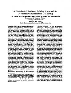
remainder of the puzzle can be solved without disturbing it. The ordering of the patches is depicted on Figure 1. Its implementation is realized with an EPS program that can compute such orders from any final situation, because we do not necessarily assume that the goal state leaves the blank in a corner. It eventually provides all the agents of the puzzle with correct dependency relationships (for more details about its functioning, see [Drogoul & Dubreuil 1992]) by giving goals to the patches. If we assume that pi > pj means that pi is placed just before pj in the ordering list, which means that:

if pi > p j & goal(Ti) = pi then goal(pj) = Ti dependency(pi ) = Tj & dependency(Ti) = pj

(17) (18)

Hence, when Ti satisfies itself, it will send a TrySatisfaction message to pj. As patches are always considered as satisfied, pj will then directly send the same message to its dependency, which will try to satisfy itself, and so forth, until the last patch in the list is reached. 4 4 4

4 3 3

4 3 2

4 3 2

4 3 2

4

3

2

1

1

4

3

2

1

Fig. 1.A

All the patches are ordered in a list by their peripheral distance to the blank in the final state (1.A). Patches at the same distance are then chained together (1.B). Finally (1.C), all these lists are linked up (the last patch in the first list with the first patch in the second list, and so forth). Fig. 1.B

Fig. 1.C

An interesting aspect of this ordering is that of the progressive reduction of the puzzle during the solving. As a matter of fact, once the top row and the left column have been positioned, the system comes back to a pseudo-initial state, with a puzzle of reduced dimensions to solve. This will help us to prove the completeness of our method and compute its complexity (Sections 7.1 & 7.3)

4

Decision-Makings of the Tiles

4.1 An Introduction to the Behaviors As stated in the section 2.2, the actions that compose the behavior of an agent must be coded according to the domain in which the agent acts. In a way, we encounter the same difficulties as those faced by heuristic search: we follow a general model of solving but we need to take the properties of the problem into account. These properties will be translated, in the EPS model, into a set of local heuristics used by the agents when they perform their behaviors. The next sections will then be devoted to the description of these heuristics. Section 4.2 presents the "Manhattan GoalBlank" heuristic used in the satisfaction and flight behaviors . And, in Section 5, we show how to improve this heuristic to definitively eliminate the occurrence of loops during the solving. 4.2 Manhattan Goal-Blank Distance (MGB) In heuristic search, the usual way to compute the "distance" between two states of the n-puzzle is to compute the manhattan distances from all the tiles to their goals, and to sum them. It gives a good approximation of the correctness of the state and never overestimates the cost of the solution. We can then assume that, from the tile's point of view, such a computation will provide it with a good approximation of the distance that separates its current state from its goal. From its local point of view, a tile only "knows" two patches: its current state and its goal. Each move of the tile, be it a move for satisfaction or a move for fleeing, will be made by sliding on a patch adjacent to its current state. The decision-making for this move will be made according to two Manhattan distance computations (grouped under the name MGB): 1. 2.

The Manhattan distance of each adjacent patch to the goal of the tile. With the aim of choosing the optimal path from its local point of view, this first distance will provide the tile with the patches nearest to its goal. The Manhattan distance of each adjacent patch to the blank. This will provide the tile with the patches nearest to the blank, enabling it to push as few tiles as possible when aggressing.

As long as there is no global entity supervising the solving, the MGB distance computations use a distributed algorithm implemented by the patches. In that way, each time a tile wants to know the distance between its adjacent patches and its goal, the goal patch is asked by the tile to generate a wave by transmitting the value 1 to its own neighbors. This wave is then transmitted to their respective neighbors with a value increased by one. Once the computation is finished, the four patches adjacent to the tile own a unique value which corresponds to their respective manhattan

distance to the goal. In the same way, each time a patch remains empty (which means it is the current blank position), it generates a similar wave, kept by the patches as their distance to the blank. The current tile that is about to move uses these distance computations for two different purposes, which respectively correspond to its satisfaction and flight behaviors: 1.

2.

In its satisfaction behavior, it chooses the patch nearest to the blank among the patches nearest to its goal. This patch, if not free, tells its tile to flee; once done, the current tile moves onto it. This aggression message contains two constraints: avoid the goal patch of the current tile, and avoid the patch of the prior satisfied tile. These two constraints, only valid for the first fleeing tile, aim at optimizing the solving. The first one prevents the fleeing tile from sliding onto the goal of the active tile. The second relies on the hypothesis that the prior active tile has reached its goal and should not be disturbed. A tile on the run will try to free its patch as soon as possible, in order to give place for the aggressor. This flight takes place in four steps: a. Remove from the possible patches the ones provided as constraints. b. If the remaining patches contain the goal of the tile, elect it. c. Otherwise, choose among the nearest patches to the blank the nearest to its goal. d. Once chosen, the patch, if not free, will ask its tile to flee.

It must be noticed that the MGB computations are used in a different way in the flight behavior than in the satisfaction behavior. During a flight, the distance to the blank takes precedence over the distance to the goal so as to reduce the number of flights. But a tile on the run will nevertheless be attracted by its goal, in order to reduce its number of moves whenever it is going to satisfy itself.

5

How to Avoid Loops ?

5.1 Basic Idea There are many situations in which loops can occur during the solving. For example, if two tiles respectively lie on the goal of each other, they will aggress each other indefinitely, according to the second step of the flight behavior. More complicated loops can occur during a solving, involving many tiles. In our system, we can then generalize by stating that loops arise when a tile agresses an already fleeing or satisfying tile. In heuristic search, loops are easily avoided when the system keeps the prior states in memory. When coming back to a previously computed state, it can then backtrack before this state and avoid the loop. This solution cannot be used in our system, because the decision making of a move only takes the local knowledge of the tile that moves into account. And that knowledge does not include any information about the global state of the problem. We then have to provide the tiles with local information that could allow them to avoid generating loops when moving. We do not want to take back the puzzle to a prior state when a loop arises, but to avoid their appearance. The distinction is important. A system that ignores loops will also ignore backtracks. And backtracks are known to be very expensive in both time and space. Our idea is close to those developped in many domains like Robotics or Artificial Life. We consider that the history and the representation of the solving is to be found on the puzzle itself. Acting in this world will then modify it, but also change the way the other entities view it. The moves of our tiles are only decided with respect to the distance computations. And these computations can be viewed, from a global viewpoint, as topographies of the puzzle in terms of declivity (a tile will be inclined to slide downwards rather than upwards towards its goal or the blank, see Figure 3). Hence, in order to avoid loops, the decision-making of one tile should have an effect on that of the following tiles by modifying this topography, thus modifiying their distance computations and, eventually, the paths they will choose. In a simplified way, we then consider that a tile about to move becomes a temporary obstacle for the others. Their respective decisionmakings will now prevent them from choosing it as a tile to aggress (directly or indirectly). 5.2 a Voronoï diagrams based MGB distance computation (VMGB) As MGB is computed by the patches in a distributed way, the easiest way to modify the topography of the puzzle is to affect the behavior of the patches, with respect to the current behavior of their tile. We then state that a tile on the move (or already satisfied) locks its patch before taking a decision. Once locked, a patch will not accept the "waves" generated by MGB. These waves will therefore now break on locked patches as they would break on obstacles. In other words, the computation of the local heuristics now prevents the tiles from aggressing satisfying or fleeing tiles. We called this distance computation VMGB because it is close to the Voronoï's diagrams used in robotics for finding paths (see Figure 3). A simple example of it is fitted on Figure 2.

4

3

3

2

2

1

1

0

2

1

4

5 B

A 9

C

6

8

Possible moves for "H"

7

X

Other patches

8

A

Tiles

10

D E

Blank

Blank patch

H

F

Tile H

Locked patch

G

Fig. 3 The same computation represented in 3-D

Fig. 2 An example of VMGB computation

A attacks B, which attackes C, etc... and H has to choose the nearest patch to the blank on which to flee. H then computes the distance between the neighbors of its patch and the blank. The wave produced by the blank breaks on locked patches. Once the patches adjacent to H have been reached, it will choose the one whose "value" is the smallest.

In that way, a tile does not take all the patches nearest to the blank into account, but only those being able to slide towards it without shifting locked patches. We then avoid loops without backtracking and without too much computations (it is easy to see that the complexity of VMGB is O(N), N being the size of the puzzle). However, sometimes, it is necessary to attack a locked patch (see section 6.2), because no other patches can be chosen. So, fleeing tiles can unlock their patches, which results in unlocking all the patches of the puzzle (by a simple propagation of the message).

6.

Examples

6.1 The solving of a 8-Puzzle We present on Figure 4 snapshots of a 8-puzzle solving. They only show the moves of the tiles that seek satisfaction. The locked tiles are the tiles that, once satisfied, will not be shifted any more. F B C E F D

G E H A D B C A H G

F G E B H A C D E B C A H F D G

A B C D E F G H

F G E H C A B D B C E A H F D G Initial State

F H B B A E

G E C D A C H G F D

F GE B H A C D

F H B A

E G D B G E F

C A C H D

A B C Goal D E F State G H

F E C B H G D A A B C G H D E F A

F E B D H A B G D E H

Current Tile

C G A C F C

E F D A D G

B C G H A B C F E H

Satisfied Tile

D

E F D A D G

B C H G A B C F E H

Locked Tile

Fig. 4 Snapshots of a solving in progress (left to right)

6.2 Solving the problem of the edges The underlying paradigm of our system is to make the solution emerge from interactions between small agents. As an instance of emergence, the solving of the problem of the edges is described in this section. The task is to satisfy a tile whose goal is an edge of the puzzle without shifting the satisfied tiles that make up the row or the column including this edge. Figure 5 focuses on the problem met above by tile A and shows the moves of the fleeing tiles, in order to see how it works. B and C are satisfied, and A tries to reach its goal. A then attacks A H A H E A H A G G H E.The patch of B is provided as a constraint during this attack. E F D G F D G F D G E F D E F D finds no patch for fleeing. It then unlocks all the patches and Fig. 5 Snapshots of the solving of the top row attacks A (the patch of B is still a constraint). A flees on the blank. Since it remains unsatisfied, it attacks E again, now with its goal as constraint. E then attacks F, which attacks D, and so on until B flees on the blank. A then slides on its previous patch and attacks B. In this case, there are no valid constraints. B then attacks C, which prefers to slide onto its goal rather than onto the blank. Therefore, it attacks H, which attacks G, which flees onto the blank. A now satisfies itself and the row is solved. E

B

C

E

B

C

B

C

B

C

H

A

B

C

7.

Theoretical analysis

7.1 Completeness The completeness of our method for any size of N-puzzle will be proved by induction on the size of the puzzle. We assume that the subgoal sequence is the same as in Figure 1 and that the lines and columns are numbered from 1 to n, starting from the blank position in the final goal state. Thus, the first tiles that will try to satisfy themselves will be those making up the line n. Theorem 1: The n-1 first tiles of line n can satisfy themselves without being shifted by an attack. Proof: It is obvious that the first tile T1 can satisfy itself and lock its patch without disturbing any previously satisfied tiles. Let us now assume that Ti (1 < i < n-1) satisfies itself without shifting previous tiles. Can Ti+1 also reach its goal? A satisfied tile Tj can be pushed out of its patch iff a fleeing tile Tf attacks it after having unlocked this patch (tiles reaching for satisfaction never unlock patches). But this cannot happen in this case: all the distance computations have taken the locked patches into account and choosing the patch of Tj would lead to a dead-end. Tf will only choose an unlocked patch that can be reached from the blank. So the path chosen by Ti+1 (and all the tiles it attacks) never passes through locked patches. Having shown that, given i satisfied tiles on line n (1 < i < n-1), T i+1 can be satisfied without shifting them and that T1 can satisfy itself, the proof of Theorem 1 by induction on i is obvious. Theorem 2: When the nth tile of line n (Tn ) seeks satisfaction, it may destroy some previous satisfactions but puts them back in place when reaching its goal. Proof: When trying to reach its goal, Tn can meet three situations: (1) Its goal is blank and adjacent to it: it just moves on it without destroying any satisfactions. (2) Its goal is adjacent to it but not free: this is the case described in Section 6.2. Some satisfactions are destroyed but, in this case, Tn inevitably attacks Tn-1. As a fleeing tile primarily chooses its goal when it is adjacent, Tn-1 will flee onto its goal patch (it can make Tn-2 flee at its turn on its goal, and so forth until all the satisfactions have been re-established). (3) Its goal is blank and there is a tile Tk between Tn and it. Tn attacks Tk with the blank as constraint. Tk cannot flee because the other patch adjacent to the blank contains Tn-1 and is locked. It then unlocks the patches and attacks the tile below Tn-1. And we are back to point 2. We are then able to place Tn when the n-1 first tiles of row n are satisfied. It is obvious to do the same proof for column n, and to show that we also solve it. As stated in Section 3, once the top row and the left column of a puzzle are solved, the remainder can be solved without disturbing them. So the system can always reduce the solving of an n x n puzzle to that of a (n-1) x (n-1) puzzle, whatever n > 1. Moreover, the 1-puzzle is obviously solved with our system. It is decomposed into one agent: a patch. The solving begins by sendingthe message trySatisfaction to this patch. As a patch is always satisfied, the solving immediately stops. As a conclusion, if we call Pn a n x n puzzle, and Pn-1 the (n-1) x (n-1) puzzle obtained by removing the top row and the left column from Pn, we have: ∀n > 1, solved(Pn) ⇔ solved(Pn-1) solved(P1)

⇒

∀n, solved(Pn)

(19)

Consequently, whatever is the size of the puzzle, the behaviors of the agents do not have to change. 7.2 Decidability A solving method is said to be decidable iff: (1) it finds the solution if there is one and stops with acceptance; (2) it stops with no acceptance when there is no solution (instead of looping). The first point is verified because the method is complete. Is there a way to verify the second point ? Theorem 3: If a satisfied tile is attacked, and if the goal of the tile that seeks satisfaction is not an edge, the puzzle can not be solved. Proof: Theorems 1 & 2 prove that satisfied tiles cannot be shifted unless the goal of the current tile is an edge. So, if a satisfied tile is attacked while the goal of the current tile is not an edge, there is something wrong with the puzzle. As a matter of fact, a wrong initial state of the n-puzzle (often generated by the transposition of two tiles) leads to an infinite loop of aggression between tiles that seek for satisfaction. As these tiles cannot satisfy themselves concurrently, it means that they alternatively reach their goal and then flee when being attacked. And that is exactly the situation to which Theorem 3 applies. Practically, a way to stop the solving in this situation is as follows: Everytime a satisfied tile is attacked, it looks at the goal of the current tile, provided as constraint with the flee message. If this goal is not an edge (i.e. a patch with only two neighbors), it does not answer the attack and the solving stops, leaving the puzzle in a wrong state.

7.3 Complexity In this part we bound the theorical complexity of our algorithm. The complexities we have studied are: (1) the space complexity SP(N) (how much room does a solving take), (2) the length of the solution LG(N) and (3) the execution time ET(N). In the following, we will call N the number of tiles (or the size) of the puzzle, n its number of columns. The relation between them is: N = n2 - 1. a) Space Complexity As our algorithm does not keep states of the problem in memory, the only space allocated is the one to the agents. So the required space is a linear function of the number of agents. As the number of agents grows linearly with the size of the puzzle (an N-puzzle has N tiles and N+1 patches) the space complexity is: SP(N) ~ O(N)

(20)

As it has been stated in Section 3, our algorithm orders the agents so as to solve successively entire rows and columns. So the solution length complexity as well as the execution time complexity will be recursively computable. That is, if RC(k) is the complexity to solve the kth row and the kth column, we can assume that the whole complexity C(n) of the solving is: n

C (n) = ∑ RC (i)

(21)

i=1

In the two following sections, we will then compute RC(n), with respect to the length of the solution and the required time, and deduce LG(n) and ET(n) from it. b) Solution Length Complexity In this section, RCM(n) represents the number of moves required to achieve the top row and the left column of an N-puzzle. In an n x n puzzle, the farthest one tile can be from its goal patch and from the blank is 2n-1 patches. So the maximum number of moves generated by its first move towards its goal is 2n-1. Thereafter, the blank will be positioned just behind it. Hence, sliding onto the remaining 2n-2 patches will at most require 5 moves each (see Section 6.1 for an illustration). Eventually, we can roughly bound the number of moves required to position a tile on an edge by 2n2 - 2 (in the worst cases, like the one depicted in Section 6.2, all the tiles have to move twice). So, the total number of moves generated by one of the 2n-3 non-edge tiles that compose the top row and the left column for reaching its goal is at most: (2n-1)+ 5 (2n-2). And that of the edge tiles is: (2n-1)+ 5 (2n-2) + 2n2 - 2. Completing the top row and the left column will then require at most: RCM(n) = (2n-3) (2n - 1 + 5 (2n - 2)) + 2 ((2n-1)+ 5 (2n-2) + 2n2 - 2) = 26n2 - 34n + 7

and so: d°(RCM(n)) = 2

(22)

n

As LG(n) = ∑ RCM (i) we can then deduce that d°(LG(n)) = 3. i=1

Since N = n2 - 1, the complexity of the solution length is at most: LG(N) ~ O( N N )

(23)

b) Execution Time Complexity Let RCT(n) represent the execution time required for solving the top row and the left column. Any move can be decomposed into the same set of actions: propagating from the blank, then from the goal, making a decision and physically moving. The execution time of the first two actions is at most K1 * (n2 - 1), where K1 is the constant amount of time used by the propagation behavior of each patch, and n 2 - 1 the maximum number of patches involved in this propagation. Making a decision and physically moving only depend on the local knowledge of the tile, and then require a constant time K2 . Consequently, the time consumed by a move is: TM(n) = 2K1*(n2 - 1) + K2. We then have the following relation: RCT(n) = RCM(n) * TM(n)

which induces that: d°(RCT(n)) = 4

(24)

n

As ET (n) = ∑ RCT (i) , we can then compute d°(ET(n)) = 5. i=1 So the complexity of the execution time is at most: ET(N) ~O(N 2 N )

(25)

8.

Experimental results

In order to verify the effectiveness of our method, we have made a wide range of tests on instances of N-puzzles. First point, our system is able to solve very large puzzles. We have made experiments on the 8 up to the 899-puzzle (30x30). For the majority of them, these are the first reported results. We have summarized them in Table 1, by indicating the average solving times, solution lengths and number of moves made by each tile. All these results have been registered by running the EcoTalk kernel written in Smalltalk-80 release 4.1 on a Sparc 10 workstation. They have been obtained by making the average over a hundred random problem instances of each size. Width (n) 3 4 5 6 7 8 9 10 11 12 13 14 15 16

Size ArevageTime Average Length Average Width (N) (seconds) (moves) moves per tile (n)

Size ArevageTime Average Length Average (N) (seconds) (moves) moves per tile

8 15 24 35 48 63 80 99 120 143 168 195 224 255

288 323 360 399 440 483 528 575 624 675 728 783 840 899

0000.22 0 000.75 0 002.48 0 004.51 0 009.66 0 017.03 0 023.15 0 035.47 0 052.76 0 065.78 0 086.72 0 106.92 0 116.48 0 165.87

00 048.90 00 142.10 00 283.00 00 482.00 00 746.30 01 109.20 01 455.20 01 947.70 02 483.10 02 889.10 03 361.90 04 199.70 04 881.50 05 581.90

6.1 9.5 11.8 13.8 15.5 17.6 18.2 19.7 20.7 20.2 20 21.5 21.8 21.9

17 18 19 20 21 22 23 24 25 26 27 28 29 30

0 204.46 0 230.69 0 271.57 0 292.02 0 340.88 0 415.12 0 477.35 0 544.91 0 625.58 0 655.03 0 782.01 0 897.64 1 036.30 1 179.58

06 267.10 06 947.60 07 797.20 09 004.70 09 882.00 11 093.70 12 404.00 13 340.10 15 181.20 16 514.00 18 496.80 19 999.40 21 229.20 23 009.00

21.8 21.5 21.7 22.6 22.5 23 23.5 23.2 24.3 24.5 25.4 25.5 25.3 25.6

Table 1 - Average results for the solving of the 8 up to the 899-puzzle

It is important to note that we do not obtain optimality in solving. The lengths of the solutions obtained for the 8 and 15 puzzles are approximatively a little more than the double of the optimal ones (respectively 22 and 53 moves, as computed by A*). While no practical techniques exist for computing optimal solutions for greater puzzles, we cannot conclude on their performances. But the system solves them in a reasonable time (less than 20 minutes for the 899-puzzle) and we suspect that it outputs a solution that is around twice the optimal. 60000 K1= 9 50000 Theoretical Complexity O(N*ˆN) 40000 N*LOG(N)/K1 30000

20000

Solution Length

10000

Puzzle Size (N)

0 0

100

200

300

400

500

600

700

800

900

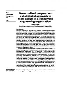
Fig. 6 - Evolution of the solution length from the 8 to the 899-puzzle

Second point, the results in both execution time and solution length are obviously much better than what was expected from the theoretical complexities. The first reason is that theoretical complexities only reflects the solving of the worst cases. The second reason is directly due to the flight behaviors of the tiles: by primarily choosing their goal if it is adjacent, they progressively reduce the disorder of the puzzle during the solving, even when they are not trying to satisfy themselves. In fact, once the top row and the left column have been solved, the remaining puzzle is much less disordered than a random instance of the same size. All the flights generated by the first tiles have reduced the average distance of each unsatisfied tile to its goal. Unfortunately, it is difficult, if not impossible, to take this property into account when computing the complexities.

The third reason is that the VMGB computation stops when reaching the adjacent patches of the tile that has generated it. In that way, most of the cases only require the propagation among ten or less patches instead of n2 , because a tile that has moved will have the blank just behind it. As is shown on the diagram of Figure 6, the dots that represent the actual solution lengths appear to be closer to the thick line that depicts the experimental complexity O(N*log(N)) than to the broken line that depicts the exact theoretical complexity. Of course, this result has to be validated on even greater sizes of N-puzzle, because 28 data points are clearly unsufficient. However, if it is verified, it would break the idea that the optimal solution length must be O(N*√N) [Korf 1990b]. 5000 K2=23 4500 4000 3500 3000 2500

Theoretical Complexity O(N2*ˆN)

2000 (N*ˆN) / K2 1500 Time (seconds)

1000

Puzzle Size (N) 500 0 0

100

200

300

400

500

600

700

800

900

Figure 7 - Evolution of the execution time from the 8 to the 899-puzzle

We obtain similar results for the execution time, whose curves are depicted on Figure 7. Instead of O(N 2 *√N), the experimental execution time complexity appears to be closer to O(N*√N). Again, it has to be validated by further experiments. But we suspect these results to be closer to reality.

9.

Conclusion

In this paper has been presented a distributed approach for solving the N-puzzle problem. This approach is based on the decomposition of a problem into the set of the smallest independent subgoals that can be described, be they serializable or not. These subgoals are at their turn decomposed into agents whose task is to satisfy the subgoal. We have chosen the Eco-ProblemSolving model for describing the internal functioning of these agents. Each of them is then characterized by a state, a goal, a satisfaction behavior and a flight behavior. Those kernel behaviors invoke domain-dependent actions that must then fit with the domain in which the agent is involved. The description of these actions has been made by presenting their basic algorithm and the heuristics used in it, namely the MGB and VMGB distance computations. A simple example of solving has been presented, followed by an example of what can be called an “emergent solution” to the problem of the corners. We then prove that the method is complete and decidable for any size of N-puzzle. Its theoretical complexity is calculated, with respect to the size of the puzzle, for three values: the room used in memory, the solution length and the execution time. Following this theoretical part, the experimental results have allowed us to show the first published results for puzzles whose size is over 800. When studying these results, we have shown that the theoretical complexity must be used carefully, because it does not appear to reflect the reality. As a conclusion, we would like to say that, although the paper only deals with the N-puzzle case, our work must not be viewed as simply the design of a special purpose system for solving it. The solving of the N-puzzle is just part of a more general project on the Eco-Problem-Solving framework, the goal of which is to elaborate a formal methodology for applying distributed techniques to problem solving. In order to verify its paradigms as quickly as possible, we chose to test this methodology on various classical toy problems. And we decided to publish the results on the N-puzzle because they had overrun our expectations. The next step will be to generalize the behaviors presented here to deal with problems close to the pebble games of [Kornhauser & al. 1985] and then with direct application in robotics.

Bibliography [Brooks 1987] R. Brooks, "Planning is just a way of avoiding what to do next", Mit Working Paper 303, 1987. [Chapman 1990] D. Chapman "Vision, Instruction and Action", PhD Thesis, MIT AI Technical Report 1204, April 1990. [Delaye & al. 1990] C. Delaye, J. Ferber & E. Jacopin "An interactive approach to problem solving"in Proceedings of ORSTOM'90, November 1990. [Drogoul & al. 1991] A. Drogoul, J. Ferber, E. Jacopin "Viewing Cognitive Modeling as EcoProblem-Solving: the Pengi Experience", LAFORIA Technical Report, n°2/91 [Drogoul & Dubreuil 1990] A. Drogoul & C. Dubreuil "EPS Implementations of classical AI problems", LAFORIA Technical Report, LAFORIA 1990 (in French). [Drogoul & Dubreuil 1992] A. Drogoul & C. Dubreuil “Eco-Problem-Solving model: Results of the N-Puzzle”, in “Decentralized AI 3”, Werner & Demazeau Eds., Elsevier North Holland, 1992, pp 283-295. [Drogoul & Dubreuil 1993] A. Drogoul & C. Dubreuil, “An EPS implementation of the Tileworld”, to appear as a LAFORIA Technical Report n°??/93 [Durfee & al. 1987] E.H Durfee, V.R. Lesser, D.D. Corkill "Cooperation through communication in a distributed problem solving network" in "Distributed Artificial Intelligence", M. Huhns (Ed) Pitman Publishing,1987. [Ferber & Drogoul 1992] J. Ferber & A. Drogoul, “Using Reactive Multi-Agent Systems in Simulation and Problem Solving”, in “Distributed Artificial Intelligence: Theory and Praxis” [Hart & al. 1968] P.E. Hart, N.J. Nilsson and B. Raphael, "A formal basis for the heuristic determination of minimum cost paths" , IEEE Trans. Syst. Sci. Cybern. 4, 1968. [Hubberman & Hogg 1988] B.A. Hubberman & T. Hogg, "The behavior of Computational Ecologies" in “The Ecology of computation", B.A. Huberman, Ed. North Holland, 1988. [Katz & Rosenschein 1988] M.J Katz & J.S. Rosenschein, "Plans for multiple agents" Workshop on Distributed Artificial Intelligence (Preliminary Papers), Lake Arrowhead USA, 1988. [Korf 1985] R.E. Korf, "Depth-First iterative-deepening: An optimal admissible tree search" in Artificial Intelligence 27, 1985. [Korf 1990a] R.E. Korf, "Real-Time Heuristic Search" in Artificial Intelligence 42, 1990. [Korf 1990b] R.E. Korf, “Real Time Search for Dynamic Planning”, Proceedings of the AAAI Symposium on Planning in Uncertain, Unpredictable or Changing Environments, Stanford, March 1990, pp. 72-76 [Kornhauser & al. 1985] D. Kornhauser, G. Miller, P. Spirakis, “Coordinating peeble motion on Graphs, the Diameter of Permutation Groups, and Applications”, Proceedings of IJCAI’85, vol.2, pp. 1034-1035, 1985. [Ratner & Warmuth 1986] D. Ratner & M. Warmuth, “Finding a shortest solution for the NxN extension of the 15-puzzle is intractable”, in Proceedings of AAAI 1986, Philadelphia, Pa, 1986.