A metaheuristic multi-criteria optimisation approach to portfolio selection

Journal of Applied Operational Research (2014) 6(4), xx–xx © Tadbir Operational Research Group Ltd. All rights reserved. www.tadbir.ca ISSN 1735-8523 (Print), ISSN 1927-0089 (Online)

A metaheuristic multi-criteria optimisation approach to portfolio selection Giacomo di Tollo 1,*, Thomas Stützle 2 and Mauro Birattari 2 1 2

Dipartimento di Management, Università Cà Foscari di Venezia, Italy IRIDIA, Université Libre de Bruxelles, Bruxelles, Belgium

Abstract. Portfolio selection is concerned with selecting from of a universe of assets the ones in which one wishes to invest and the amount of the investment. Several criteria can be used for portfolio selection, and the resulting approaches can be classified as being either active or passive. The two approaches are thought to be mutually exclusive, but some authors have suggested combining them in a unified framework. In this work, we define a multi-criteria optimisation problem in which the two types of approaches are combined, and we introduce a hybrid metaheuristic that combines local search and quadratic programming to obtain an approximation of the Pareto set. We experimentally analyse this approach on benchmarks from two different instance classes: these classes refer to the same indexes, but they use two different return representations. Results show that this metaheuristic can be effectively used to solve multi-criteria portfolio selection problems. Furthermore, with an experiment on a set of instances coming from a different financial scenario, we show that the results obtained by our metaheuristic are robust with respect to the return representation used.

Keywords: portfolio selection; multi-criteria; metaheuristics; mean-variance; index tracking; return computation * Received January 2014. Accepted June 2014

Introduction Portfolio selection is about choosing, out of a given universe of assets, which asset to invest in and by how much so that, for a given required return, the corresponding risk is minimised (Markowitz, 1952). Amongst portfolio selection paradigms, active portfolio selection requires the investor to produce the estimates about future returns. Contrarily, when the investor aims at constructing a portfolio that replicates the behavior of a stock exchange index, we have the paradigm of passive portfolio selection. Most work about portfolio selection relies on the Markowitz model (i.e., optimising w.r.t. return and variance, see Markowitz (1952)). Indeed, it has been shown that just focusing either on return or on risk does not capture all relevant information required by investors to make their investment choice (Baker and Haslem, 1974). Other attributes have to be incorporated, either to embed personal investor’s opinions, or to face with specific investment constraints and to discriminate amongst investment alternatives. With reference to this latter point, it is a common idea that a single dimensional risk measure (in our case, the variance) is not sufficient, due to the fact that the investment’s return variability *Correspondence: Giacomo di Tollo, Dipartimento di Management, Università Cà Foscari di Venezia, San Giobbe - Cannaregio 837 - 30121 Venezia, Italy. E-mail: [email protected]

G di Tollo et al

3

(and subsequently, the investor’s notion of ‘risk’) can be due to several measures related to the financial and economic conjuncture (Hallerbach and Spronk, 2002). For this reason, other criteria have to be taken into account, replacing the return-variance approach with a multi-dimensional risk concept: depending on the specific circumstances of the investor, a specific set of criteria may be relevant. Furthermore, in the last years a debate is spreading opposing standard investors, whose utility functions just take into account the portfolio’s return, and non–standard investors, whose utility functions take into account additional criteria. The reason for taking into account additional criteria can be manifold: it can be related to non -financial requirements (for example, to embed preferences, or to help the environment), or it can be related to a mistrust of data used to assess the asset’s return. In these cases, the choice of introducing a further objective is straightforward, and amongst the objectives, the tracking error has been proposed by Steuer et al. (2005): passive and active approaches, who are generally referred to as mutually exclusive and not used in conjunction, have already been suggested to be used together, to embed user’s preferences and to give more explanatory power to the resulting model. Indeed, there exist valid reasons to optimise jointly return, variance and tracking error, and combining active portfolio selection with index tracking has been suggested by Jorion (2003). Nevertheless, up to the authors’ knowledge, works that combine active and passive approaches do not provide a wide perspective on the motivation beneath their approaches, and their experimental setting is not built in a consistent way regarding algorithm strategies used, algorithm parameter tuning, and descriptions of their outcomes (Roman et al. (2007)). In Burns (2003), tracking error and Sharpe ratio are optimised; Yu et al. (2006) use index tracking and downside risk, treated as a convex optimisation problem and solved by convex programming algorithms. Multi-objective portfolio selection problems have been deemed to be computationally untractable given the investor’s specific decision context (see Arthur and Ghandforoush (1987)), and just few works have been proposed to draw the efficient non-dominated set: the main approaches focus either on goal programming (see Spronk and Hallerbach (1997) for an overview), on models devised to embed decision-makers preferences and to determine the optimal portfolio (Ballestero (1998), Ehrgott et al. (2004), L’Hoir and Teghem (1995)) or on linearisation of the model (Xu and Li (2002), Zopounidis et al. (1998), Ogryczak (2000)). Metaheuristics are search strategies to guide the behaviour of subordinated heuristics, and they have been successfully applied to many portfolio selection problem formulations (di Tollo and Roli, 2008). They have been proven to be effective in dealing with multi-objective combinatorial optimisation problems, but their application to active-passive multi-criteria portfolio selection is still limited: few works have been dealing with the topic, notably Thomaidis (2010), who adopts simulated annealing, genetic algorithms and particle swarm optimisation; and Vassiliadis et al. (2009), who apply ant colony optimisation to an active–passive approach under a downside risk framework. Again, they focus on generating one (or very few) non-dominated point(s) in the objective space but they do not generate a good approximation to the whole Pareto frontier. In our work, instead, we want to generate an approximation of the whole Pareto set for multiobjective portfolio selection problems. Up to the authors’ knowledge, this is the first time such an attempt has been done. We also want our approach to be robust w.r.t. the data representation: It is recognised that when tackling an optimisation problem, we make approximation errors (von Neumann and Goldstine, 1947). In our case, a possible source of error is the translation of the real problem to the model. For example we want to convert actual prices, which are thought to be continuous, to their mathematical description, which has to be discrete. Converting prices to returns can be done in different ways. For instance, one can consider discrete or continuously compounded returns, which are different from a theoretical point of view, and represent two possible options to translate the real world into a mathematical model. From a theoretical point of view, results should be sensitive to the returns’ representation chosen (Acker and Duck, 2007); Dimitrov and Govindaraj, 2007), but practically we want approaches that are robust w.r.t. different input representations (Gilli and Schumann (2010)). In our work, we introduce an approach that is robust with respect to imprecise and noisy data, and we show that our approach is not sensitive to the choice of a continuous or discrete return representation. Thus, we can summarise our reasoning as follows: there is a conceptual difference between the discrete and the continuous return representation, but when implementing them to translate historical data into our optimisation problem, we see that the metaheuristics used do not show different behaviour on the two cases, since the computation times and the obtained portfolios are similar, and there is no problem of sensitivity, since there is no perceivable difference over the ordinal distributions of portfolios

4

Journal of Applied Operational Research Vol. 6, No. 4

returns. Thus, the goals of this paper are: to devise a multi-criteria formulation combining active and passive portfolio selection approaches; to solve the resulting problem by means of metaheuristics and to show that the devised approach is not sensitive to the return representation used. The article is structured as follows: portfolio selection theory will be briefly discussed in the next section, before describing the proposed multi criteria approach in section 3. Section 4 will describe the algorithms used, and the experiments based on the two return representations will be introduced in section 5. Results are analysed and compared with results obtained on instances from a different financial scenario on section 6. The paper is concluded by a summary and proposal for future works.

Portfolio selection As a common hypothesis in portfolio selection, information about future asset prices is contained in their historical prices, and returns are treated as stochastic variables. In the most common approach, returns are treated as normally distributed, and for each asset i the asset expectation is given by its return average ri, and its risk by return variance σi2 (or its standard deviation σi). Given a universe U composed of n assets, different assets are held together to form a portfolio, i.e., a vector X whose i–th element represents the fraction of the total wealth invested in asset i (1 ≤ i ≤ n). Let ri,t be the return of asset i at time t, Si,t be the price of asset i at time t and σij be the covariance of returns on assets i and j. Returns are drawn from prices, and we consider that they can be computed in two different ways: either continuously compounded, so that ri,t = lnS i,t S i,t 1  , or discretely compounded, so that ri,t = Si,t  Si,t 1  Si ,t 1 . The expected return of n n n r x and its return variance is  2p = the portfolio is r p =  x x . Other risk measures can be used to assess i =1 i i i =1 j =1 ij i j portfolio’s risk, see di Tollo and Roli (2008) for an overview. t



 

The Markowitz model The Markowitz model is the main specimen of active portfolio selection approaches, and it is stated as follows: n

min

n



(1)

ij xi x j

i =1 j =1

Subject to n

r x

i i

 re

(2)

i =1 n

x

i

(3)

=1

i =1

xi  0

i = 1,, n

(4)

The objective function is the variance σp2 whilst re represents the minimum required portfolio return. Eq.(3) represents the budget constraints, and Eq.(4) ensures that only long positions are taken. By solving the problem for a set of values of re, it is possible to estimate the efficient frontier for the Markowitz unconstrained problem (UEF). Then, the investor can choose the portfolio depending on specific risk/return requirements. The UEF is composed of Pareto optimal solutions, i.e., portfolios such that no criterion can be improved without deteriorating any other criterion: in our example, a portfolio s is said to be efficient if there is no other portfolio u such that ru > rs and σu≤σs, or ru ≥ rs and σu < σs.

G di Tollo et al

5

Index tracking The passive portfolio selection approach states that a portfolio should achieve roughly the same return as a specified financial index (benchmark) through investing in a subset of the benchmark. Contrarily to active approaches, no estimate about returns has to be made. Let U be the universe set containing n assets; let ri,t be the return of asset i ∈ U at time t, rI,t be the return of index I at time t, xi,t be the quantity of asset i held at time t and Si,t be the price of asset i at time t. The portfolio value at time t is n

vt =

x

i ,t

(5)

 S i ,t

i =1

Given an time horizon T, the goal of the index tracking problem is to find a portfolio whose returns rp,t ( rp ,t = i =1( xi ,t  ri ,t ) , i ≤ t ≤ T) are as close as possible to rI,t, yet without full replication and having no knowledge on the index composition. This is done by penalising portfolio’s return deviations from the index, by means of minimising the following objective function (Maringer and Oyewumi (2007), Gilli and Këllezi (2002)):



T

( TE =



1

| rp,t  rI ,t | ) 

t =1

T

(6)

The parameter α scales the penalty of deviations, and different values of α lead to different optimal solutions. This formulation, referred to as “single-point index tracking problem” is common in portfolio optimisation (di Tollo and Roli (2008)), and it has also been used in multi criteria portfolio choice by Roman et al.(2007). For an outline on other objective functions, we forward the interested reader to Dahl et al. (1993), Franks (1992), Lobo et al. (2000), Roll (1992), Toy and Zurack (1989), di Tollo and Roli (2008). A multi-criteria approach for portfolio choice As a variant of the index tracking problem, let us consider the index beating problem, in which the goal is to find a portfolio that outperforms the benchmark index over time: in this situation, the objective is to maximise the excess return (difference over time between rp and rI). It has been shown that just focusing on excess return leads to inefficient results (Roll, 1992), as the risk of the portfolio is always bigger than the index one. A remedy to this situation would be to optimise the excess return and to add a constraint over the tracking error. However this approach has the shortcoming that the solution is independent from the index (Jorion, 2003); furthermore, the obtained portfolios are never efficient in terms of mean-variance analysis, as increasing the allowed tracking error leads to a volatility increase. This is due to the focus on excess return instead of total return. In order to overcome this shortcoming, a constraint on the portfolio variance has been introduced by Jorion (2003), in which three criteria are taken into account: variance, index tracking and excess return. It has been shown that the joint use of these three variables is useful when the benchmark is inefficient, leading to a consistent risk decrease at the cost of a negligible return loss: this motivates a situation in which active approaches and passive approaches are not mutually exclusive, and have to be used in a hybrid approach. There is another justification for combining active and passive approaches, which relies on the concept of enhanced index tracking (Li et al. (2011)), in which the investor has to both imitate the index by minimising the tracking error, and outperform the index by maximising the excess return. Anyhow, the approaches proposed to solve it (Canakgoz and Beasley (2009), Dose and Cincotti (2005), Gaivoronski et al. (2005), Wu et al. (2007)) are unable to identify all solutions belonging to the non-dominated set, finding just the ones located on the convex part of the Pareto frontier. These two considerations have been the motivation to improve Jorion’s concept of tracking error constrained active portfolio optimisation (Jorion (2003)) by introducing a multi-criteria approach that combines index tracking and the Markowitz model. In our approach, the absolute return will take the place of excess return because they are equivalent from a computational point of view and because this overcomes the previously stated shortcoming outlined by Jorion himself. We are solving the problem by means of a metaheuristic approach to approximate the Pareto frontier. In this way, the proposed approach is able to reflect several degrees of investors’ attitude toward risk and their trust in the market.

6

Journal of Applied Operational Research Vol. 6, No. 4

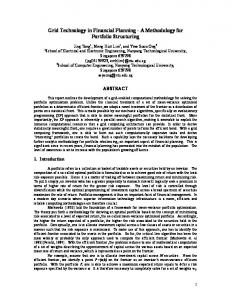
Problem definition Our main idea is to integrate the index tracking within the mean-variance framework, leading to a multi-criteria formulation whose objectives are to minimise risk, maximise return and minimise tracking error. In the following, we will use mean return as return measure, variance as a risk measure, and the formula introduced in Eq. (6) (α=1) is quantifying the tracking error. To have an idea about how these three measures are related, we show in Fig. 1 the frontier for the Markowitz’s unconstrained problem. On the x-axis we plot the portfolios’ return; on the y-axis, the upper plot shows the portfolios variance, the bottom plot shows the tracking error computed on the corresponding portfolios. It is clear that tracking error and variance are conflicting criteria, same as for variance and return.

Fig. 1. Return, variance and tracking error, instance 2, continuous. On the x-axis we plot the portfolios’ return; on the y-axis, the upper plot shows the portfolios variance, the bottom plot shows the tracking error computed on the corresponding portfolios.

Unconstrained formulation Let T be the number of observations in the time horizon, n be the number of assets in the universe, xi be the fraction of the portfolio to invest in asset i, ri,t be the return of asset i over time t, and rI,t the index return at time t. In our approach we want to minimise the variance, while constraining return and tracking error in the formulation, by imposing a minimum required return re and a maximum allowed tracking error, TE. The formulation of the problem becomes the following: n

min

n



ij xi x j

(7)

 re

(8)

i =1 j =1

Subject to n

r x

i i

i =1

n

x

i

(9)

=1

i =1

n

|(

x r

i i ,t )  rI ,t

| TE t

(10)

i =1

xi  0

i = 1n

(11)

This formulation can be solved by Quadratic Programming, and by solving the problem for different pairs of (re, TE) we obtain a three dimensional surface, which is composed of points that are non-dominated and that compose the Approximated Unconstrained Efficient Frontier (AUEF). Please notice that we are not concerned to selecting what portfolio to choose out of the AUEF, nor to define a decision-making approach able to deal with the user preferences: as for other multi-objective problems, the user will select his preferred portfolio w.r.t. an external criterion.

G di Tollo et al

7

Constraints We impose real-world constraints on the problem formulation. These are on the size of the position on each asset and on the number of assets to be held in the portfolio. Other constraints can be handled by our algorithm, such as constraints on liquidity and pre-assignment constraints (Di Gaspero et al., 2011), but they are not taken into account in our experimental phase. Cardinality constraint

Portfolio managers are usually constrained to invest in a much smaller number of assets than the hundreds or even thousands of assets that might constitute an index (Gilli and Këllezi, 2002). Let Z be the set of variables zi= 1...n, where zi=1 means that asset i is included in the portfolio, and zi=0 means it is not. The cardinality constraint imposes that the portfolio must contain at most k assets. This constraint is given by: n

z

i

k

(12)

i =1

Floor and ceiling constraints

Floor constraints are introduced to avoid small trades, and a ceiling constraint can be introduced to avoid exposure to a single asset. We set a minimum εi and a maximum δi for each asset i, such that either zi = 0 (which imposes xi = 0), or zi = 1 and we have xi ≥εi and xi ≤ δi. This is expressed as follows: εi zi ≤ xi ≤ δi zi

(13)

Constraints (12) and (13) are added to the Unconstrained formulation (Eqs .(7)-(11)) in order to obtain our constrained formulation for the multi-criteria portfolio selection problem. This is the formulation that we are taking into account in the experimental phase. By solving the problem for different pairs of (re, TE) we obtain a three dimensional surface, which is composed of non-dominated points and that compose the Approximated Constrained Efficient Frontier (ACEF). We want to stress that the introduction of a maximum cardinality constraint makes the portfolio selection problem become NP-complete, as proven by Bienstock (1996), justifying also the potential usefulness of metaheuristics for solving the problem.

Solution strategies: metaheuristics In this section, we outline the search strategies used to solve our problem. In our formulation the problem is composed of both discrete (zi) and continuous (xi) variables, hence we devise a procedure consisting of two separate methods to deal with the two variable classes. Our solver is based on the same approach introduced by Di Gaspero et al. (2007), operating a master-slave decomposition that combines a local search metaheuristic as master solver with a Quadratic Programming procedure as slave solver: a metaheuristic is used for selecting assets to be included in the portfolio. At each step it resorts to a Quadratic Programing (QP) solver for computing the best asset allocation, using as input assets only those provided as input by the master procedure. In other words, at each step a metaheuristic decides which assets are in the portfolio; then the QP solver is invoked in order to compute the optimal portion of each asset and the objective function of the current state. The resulting portfolio is accepted or not depending on the acceptance criterion implemented by the local search at hand, and the search process continues. In the following, we summarise the main local search features.

8

Journal of Applied Operational Research Vol. 6, No. 4

Search Space The search space S for the metaheuristic module is composed of the 2n possible configurations of Z (the set of discrete variables). The QP solver receives as input assets included in the state under consideration and produces optimal values to the corresponding xi variables. Neighbourhood relations Three neighbour relations are introduced: addition, deletion and replacement of one asset. A move between portfolios is identified by a pair (i ≠ j) , where i is the asset to be inserted and j the one to be deleted. In detail:   

0 < i  n, j = 0, identifies addition (asset i is added to the portfolio);

i = 0, 0 < j  n, identifies deletion (asset j is removed from the portfolio); 0 < i  n, 0 < j  n, identifies replacement (asset i is added and asset j is removed).

Initial solution Results have shown to be insensitive to the initial solution, so we start from a random initial solution feasible w.r.t. Constraint (9). Solution techniques To implement our solver, we devised a combination of Local Search and Quadratic Programming, and in this section we outline briefly both. As local search techniques, we used Steepest Descent (referred to as SD), First Descent (referred to as FD) and Tabu Search (referred to as TS). Steepest and first descent

A local search algorithm starts from an initial solution and enters into a loop that navigates over the search space, moving from the current state to one of its neighbours. In both, First and Steepest Descent, a neighbour of the current solution is selected, compared to the current solution and accepted if its cost function is better than those of the current state, otherwise the search process stops. The difference between the two approaches is in the exploration of the neighbouring solutions. In Steepest Descent all neighbours of the current solution are evaluated, and the best (w.r.t. cost function) is selected; in First Descent, the first improving solution found in the neighbourhood examination is selected (ties are broken randomly). Tabu search

Tabu search uses an additional memory to perform the search: at each step, only a subset of neighbours is explored, and the best neighbour is accepted as the new current solution. To enhance exploration capabilities, a tabu list is used, which determines forbidden moves: in this list, recently accepted moves are stored. This list can be static, if moves are forbidden for a pre-fixed time, or dynamic, if for each move a forbidden time belonging to an interval [lmin, lmax] is randomly generated. For TS we use a dynamic-size tabu list and we search for the next state by exploring the full nontabu neighbourhood at each iteration.

G di Tollo et al

9

Quadratic programming

Quadratic Programming (referred to as QP) is used to determine the best wealth allocation amongst assets provided as input by the local search procedure. To this extent, we use the Goldfarb and Idnani dual set method (Goldfarb and Idnani, 1983), which works for positive definite programs. The method starts from an unconstrained solution for the QP, which is both a dual feasible point and a primal optimal point for a subset of constraints of the original problem (i.e., an empty set). The algorithm operates till primal feasibility (i.e., dual optimality) is achieved, while maintaining the primal optimality (i.e., dual feasibility) of intermediate subproblems. These subproblems are identified by an activeset containing constraint to be satisfied as equalities by the current solution estimate. Though active-set methods are not deemed to be state-of-the-art techniques for Quadratic Programming, they are shown to achieve as good performances as more sophisticated techniques, expecially when dealing with dense matrices such as the ones at hand. Furthermore, such a strategy can be used, without being coupled with a local search approach, as a stand-alone method for the unconstrained portfolio selection problem. The First Descent (FD), Steepest Descent (SD), and Tabu Search (TS) metaheuristics have been coded in C++ exploiting the framework EasyLocal++ (Di Gaspero and Schaerf (2003)) , the QP solver has also been coded in C++ and is publicly available through the website http://www.diegm.uniud.it/digaspero/, accessed 21 December 2013. The executables were obtained using the GNU C/C++ compiler (v. 4.0.1). Most codes have been implemented by Luca Di Gaspero and Andrea Schaerf and were kindly provided to us by the authors. FD and SD have no parameter to be set; for TS we tuned its parameters by means of a statistical technique called F-Race (Birattari et al. (2002)) and found that the algorithm is very robust with respect to the parameter setting. We randomly set the tabu list size in the range [3,10] and we stopped the execution of TS when a maximum of 30 iterations without improvement is reached. Approximating the Pareto front Since our attempt is to draw the ACEF, we have devised a reactive procedure in order to produce the Pareto front. By solving our problem for an arbitrarily large value of TE, we obtain the mean-variance efficient frontier. Hence, the stricter the constraint on the tracking error, the more different become the results w.r.t. the unconstrained case. Let rmrp be the return of the portfolio obtained by minimising the variance without additional constraints, and let rmax be the maximum return amongst assets. We have determined 100 equally distributed values of the expected return re belonging to the range [rmrp,rmax]. Let rej be the j-th element in this sequence. We have then determined an increasing sequence of 100 TE values in the range [1,100]. Let TEi be the i-th elment in this sequence. For each couple we set the corresponding re and TE values in Eq. (8) and (10). Starting from i=1 and j=1, the algorithm attempts to solve the resulting optimisation problem, no matter the strategy used. The solution is added to the Pareto front, the i value is incremented and a new optimisation process is attempted. This cycle is repeated until the optimisation process gives us as a solution, a portfolio which is already in the Pareto front: if this is the case, it means that Constraint (10) is no longer binding and by increasing the i value we would obtain always the same portfolio. Hence the portfolio is discarded and a new optimisation process is attempted by setting TE=TE1 and re=rej+1. Dataset and experimental settings We used five instances from the repository ORLIB (Beasley et al. (2003)), which refer to five Stock Exchange indices. These instances represent 290 weekly observed asset prices for each asset and index value over the period 1992-1997. As said in the introduction, our goal is to devise an approach that is robust w.r.t. the data representation. Thus, in order to tackle our formulations, prices have been converted to returns using both discrete and continuously compounded formulas, in order to understand whether the diverse formulas lead to different optimisation results. Table 1 shows our benchmark features (origin, cardinality, and average variance) when using both continuous and discrete computations.

10

Journal of Applied Operational Research Vol. 6, No. 4

Table 1. Five benchmark time series from ORLIB representing stocks from 5 countries over the period 1992-1997.

Inst.

Origin

Assets

Avg. Variance (cont.)

Avg. Variance (disc.)

1 2 3 4 5

Hong Kong Germany UK USA Japan

31 85 89 98 225

0.0068 0.0059 0.0052 0.0055 0.0020

0.0084 0.0066 0.0056 0.0050 0.0023

Please notice that other instances will be introduced in following sections in order to verify whether the conclusions drawn using these instances hold. As for the constraints, accordingly to Gilli and Këllezi (2002) we have set k=10, εi = 0.01 and δi = 1. Experiments were run on a cluster with AMD Opteron 2216 dual core CPUs running at 2.4 GHz with 2x1 MB L2 cache and 4 GB of RAM under Cluster Rocks distribution built on top of CentOS 5.3 Linux.

Experimental analysis In the following, we discuss the experimental results. First we will detail the correlation analysis made before the optimisation, and afterwards we will enter into the details of the algorithm’s results. Correlation analysis Before running the solver, we performed a correlation analysis to avoid optimising criteria that are highly correlated. We computed the Spearman’s rank-based pairwise correlation (Spearman (1904)) amongst return, variance and the tracking error over a randomly generated sample composed of 1000 portfolios with random cardinality. Results are shown in Table 2. It can be seen that the correlations over the two return computation cases (continuous and discrete) are of comparable magnitude and negligible when analysing and ; conversely, higher correlation values are found for the pair , whose all values are higher than 0.48. Table 2. Random portfolios: pairwise rank based correlation analysis between pair of criteria indicated between parenthesis found when using both discrete and continuous return computation.

Continuously compounded returns

Discretely compounded returns

Inst

(TE ,  2 )

(TE , rp )

( 2 , rp )

(TE ,  2 )

(TE , rp )

( 2 , rp )

1 2 3

0.48 0.57 0.73 0.80 0.57

 0.042  0.13 0.02 0.01  0.33

 0.06  0.12 0.15 0.26  0.49

0.48 0.57 0.74 0.80 0.74

0.07  0.14 0.02 0.06  0.26

 0.17  0.07 0.14 0.24  0.29

4 5

Algorithm results In this section, we are going to discuss the results obtained by solving the multi-criteria portfolio selection formulation by the three algorithmic strategies outlined in pervious sections. First, we discuss the computational time, and then we outline the number of equal points found by the different strategies, before we conclude by analysing the coverage measure in order to assess the relative performance of the algorithms.

G di Tollo et al

11

Computation time

The computation time required by each strategy on each instance is shown in Table 3, for both continuous and discrete representations. We report times relative to the computation of the efficient frontier found w.r.t. TE=6. Running times using different thresholds are of comparable magnitude and are available upon request. The computation times are reasonable for both the continuous and the discrete case, without a clear difference between these two cases. The least time-consuming strategy is generally FD+QP, which is, as we will see in what follows, the worst performing from a solution quality perspective, whilst the most time consuming is TS+QP. We also remark the impact of the instance size: obviously instance 1 requires the smallest amount time due to the smallest number of assets contained therein, whilst instance 5 requires less time to terminate because no feasible solutions are found on many occurrences. Table 3. Computation time assessed in seconds. For each cell the first number represents the time needed to solve the continuous instance column by using strategy row; the second number represents the time needed to solve the discrete instance column by using strategy row.

Strategy

Instance 1

Instance 2

Instance 3

Instance 4

Instance 5

FD+QP SD+QP TS+QP

7 / 11 16 / 31 169 / 194

17 / 15 1105 / 1358 1409 / 1781

52 / 109 893 / 948 1271 / 1481

169 / 249 1132 / 1272 1619 / 1737

1219 / 1094 1132 / 1281 1175 / 1290

It is interesting to compare the computation times observed for our experiments and the ones obtained by tackling the bi-objective mean-variance formulation used by Di Gaspero et al. (2007). If we take into account the number of objective function evaluations, when considering the same search strategy applied to the same instance, the difference of evaluations between the mean-variance and the three criteria formulation is at most a factor of 1.23, obtained when applying SD+QP to Instance 1. These numbers are obtained by setting TE=6 and solving our formulation for the whole 100 re points, including the dominated points and not taking into account the mechanism for avoiding to generate dominated points described in previous sections. No significant differences arise between the continuous and discrete return computation schema, nor amongst using different TE values. Table 4. Computation time assessed in seconds needed for drawing the bicriteria and three criteria single TE value (TE=6). For the latter, also dominated points have been produced. The row Instance i (IT / MV) represents the ratio between the computation time required for formulation IT and the one required for MV, by the required strategy over instance i.

FD + QP

SD + QP

TS + QP

Instance1 MV Instance1 IT Instance1 (IT / MV)

1 3 3

3 12 4

187 1003 5.4

Instance2 MV Instance2 IT Instance2 (IT / MV)

9 20 2.2

14 185 46.25

534 2369 4.4

Instance3 MV Instance3 IT Instance3 (IT / MV)

10 30 3

16 347 21.6

547 5527 10.1

Instance4 MV Instance4 IT Instance4 (IT / MV)

11 362 32.9

19 463 24.3

668 6812 10.19

12

Journal of Applied Operational Research Vol. 6, No. 4

However, in terms of computation times (seconds), the differences are much larger and an indication is given in Table 4, where we show the time needed for computing the approximated efficient frontier for both the bi-criteria (mean-variance formulation, labelled as MV) and three criteria version (labelled as IT), using TE=6 (again, the whole frontier, also taking into account the dominated points). The row Instance i (IT / MV) represents the ratio between the computation time required for formulation IT and the one required for MV, by the required strategy over instance i (i ∈ [1,2,3,4]). We do not show results obtained for Instance 5, since the points obtained by IT are too few and a comparison with the MV ones is not worthwile. Only the results for the discrete return representation are shown, since the continuous one leads to comparable results. We remark that by using the IT formulation, the constraint matrix handled by the QP solver is bigger, leading to much higher computational times. By comparing the IT computational time with those reported in Table 3, we can conclude that the reactive procedure outlined in previous sections leads to a considerable time gain. Number of equal points

In Table 5 we show, for each pair of , the number of non-dominated solutions found, for both continuously compounded and discrete return formulations. Table 5. Number of portfolios found. For each cell , the first number represents the number of portfolios found by strategy row solving continuous instance column; the second number represents the number of portfolios found by strategy row solving discrete instance column.

Method

Instance 1

Instance 2

Instance 3

Instance 4

Instance 5

FD+QP SD+QP TS+QP

153 / 196 211 / 153 162 / 213

209 / 129 213 / 137 218 / 151

142 / 144 150 / 146 159 / 142

109 / 125 153 / 109 149 / 107

1/4 1/5 1/1

As a first performance measure, we pooled together the portfolios found by pairs of strategies, determining the number of equal points as the subset of portfolios that are identical for the three search strategies. The measure can be expressed as follows: let A denote portfolios found by strategy S1 and B denote portfolios found by strategy S2: the fraction of equal points between S1 and S2 is given by ((A  B)/(A  B)). Pairwise comparisons for every possible combination of runs are made and averaged. Figure 2 shows the average fraction of equal points (percentage) in the continuous and the discrete case.

(a)

G di Tollo et al

13

(b) Fig. 2. Average fraction of equal points. The plot (a) gives the results for the continuous, and (b) refers to the discrete. Coverage measure

The percentage coverage measure is used to assess the performance of an algorithm with respect to another. It says how many points of one non-dominated set are dominated by points belonging to another non-dominated set. In Table 6, we show the average percentage coverage measure over the runs for each pairwise comparison for the five instances. The value v associated to the pair indicates that v% points of the non-dominated set obtained by the strategy indicated in row is dominated by points belonging to the non-dominated set found by the strategy indicated in column. Table 6. Mean Percentage Coverage Measure, for each couple of strategies, the first column represents the continuous case and the latter the discrete.

Instance1 FD (cont) (disc) FD SD TS

Instance2

SD

TS





(cont) 9.82

(disc) 1.47

0.73 0.67

0.45 1.63

0.51

0.12





(cont) 9.12 0.12

(disc) 1.49 0.60





FD (cont) (disc)



(cont) 10.45

(disc) 12.01

0.63 0.29

0.45 0.42

0.41

0.52

FD SD TS





1.36 0.62

0.26 0.06



0.28

TS (disc) 0.94



0.52





(cont) 15.52 0.72

(disc) 1.92 0.41





Instance4

SD (cont) 0.70

TS



Instance3 FD (cont) (disc)

SD

(cont) 0.79 1.19



(disc) 0.79 0.35



FD (cont) (disc)

SD





(cont) 11.25

0.25 0

2.58 12.58

0



TS (disc) 0.38 13.01



(cont) 12.04 0.71



(disc) 0.69 2.4



FD+QP is the worst performing strategy: it shows the highest percentage of points covered by the other strategies in both the continuous and discrete case. When dealing with the discrete case, SD+QP performs better than TS+QP, suggesting that the more complex tabu search approach is not needed in our case. Observing the continuous case, we have instead that SD+QP performs rather similar to TS+QP. Anyhow, most of the times the coverage measure

14

Journal of Applied Operational Research Vol. 6, No. 4

(SD+QP vs TS+QP) is very small, and SD+QP is usually faster. Hence, we recommend its use for practical purposes. As a conclusion, we see that many pairwise comparisons between strategies lead to coverage measures which are really small. This is justified by the fact that Pareto sets are often mutually non–dominated or, as seen in the pervious section, they contain many common points. In the light of the considerations made so far (computation time, coverage measure, equal points), SD + QP is the recommended strategy: it performs well (when not even better) compared to TS+QP, at a lower computation time. This can be justified by the fact that, apart for instance 5, instances at hand are not hard to solve.

Analysis of results In this section, we analyse the results of our experimental analysis using the results obtained by SD + QP, which is the recommended technique and we are not considering instance 5 throughout this analysis as the portfolios found are few and far between. Pareto front analysis We show in Table 7 the pairwise, rank-based correlation amongst the three objectives over non-dominated points of the 5 instances as found with the different strategies. For this analysis only one run has been taken into account. First, we can see that there are strong differences between randomly generated (Table 2) and optimised portfolio’s correlation values (Table 7): correlations for and generally assume low values over random portfolios, while they are stronger correlated for optimised portfolios. Then, we see that in some cases the correlation analysis leads to different results when tackling the two different return computation approaches: for instance, in the continuous case the correlation over the pairs and obtained on instance 3 are considerably lower than on all other instances. This indicates that computing the returns in the two different ways can lead to somewhat different optimisation results, which can be seen also by visually comparing the continuous ACEF (Fig. 3 (b)) with the discrete one (Fig. 3 (c)). In the subplots of Fig. 3 we have drawn, jointly to the ACEF obtained with the settings discussed in pervious sections, the AUEF obtained by solving the unconstrained formulation (no cardinality nor floor and ceiling constraints), in order to show the higher value of variance and the unfeasible areas induced by imposing these constraints. Anyhow, by visual inspection, we can conclude that the two return computations do not lead to big differences in the frontier surface shape: in both, discrete and continuous instances the efficient points are stepwise distributed in the first part of the frontier, then they collapse into a linear structure after a given tracking error threshold. Table 7. Optimised portfolios: rank based correlation analysis between pair of criteria indicated between parenthesis found when using both discrete and continuous return computation.

st.

FD+QP

SD+QP

TS+QP

FD+QP

2 ( TE ,  ) Continuous

1

4

0.90 0.51  0.01 0.49

0.89 0.51  0.01 0.48

5

-

0.09

-

3

TS+QP

2 ( TE ,  ) Discrete

0.88 0.58 0.01 0.41

2

SD+QP

0.93 0.61 0.92 0.90 0.95

0.92 0.66 0.90 0.86 0.50

0.92 0.67 0.90 0.90 0.80

G di Tollo et al

st.

15

FD+QP

SD+QP

( TE , 1

4

0.89 0.72 0.04 0.42

5

-

2 3

2 3 4 5

0.99 0.96 0.99 0.99 

FD+QP

) Continuous

0.91 0.69 0.03 0.51  0.25 (

1

rp

TS+QP

( TE ,

0.91 0.68 0.02 0.50 1

0.94 0.71 0.92 0.90 0.95

rp  2 , ) Continuous

0.99 0.95 0.99 0.99 0.18

SD+QP

0.99 0.97 0.99 0.99 1

) Discrete

0.94 0.76 0.91 0.86 0.50 (

0.99 0.95 0.99 0.99 0.18

rp

TS+QP

0.93 0.77 0.91 0.90 0.80

rp  2 , ) Discrete

0.99 0.97 0.99 0.99 1

0.88 0.73 0.87 0.83 1

The difference between correlation values can be understood by plotting bi-dimensional representations of Pareto frontiers through bi-dimensional plots. In Fig. 4 we show the trade-off between tracking error and return (Fig. 4 (a), (b), (c) and (d)) and the trade-off between tracking error and risk (Fig. 4 (e) and (f)) for some instances, for the continuous and the discrete case (trade-off between risk and return is not provided, as for each instance the bi-dimensional plot results in portions of mean-variance frontiers overlapping to each others). Let us take into account the trade-off between tracking error and return over optimised portfolios for instance 3, in both continuous (Fig. 4 (a)) and discrete (Fig. 4 (b)) cases. It can be seen that, for each level of the tracking error, there exist many points with different return values (this is the trend generally followed in every instance) and this phenomenon is common to both figures. Nevertheless, in the continuous version, there are more low-return points associated to high-tracking error values, leading to a lower correlation value for that instance.

(a) Instance 1, continuously compounded returns.

(b) Instance 3, continuously compounded returns.

16

Journal of Applied Operational Research Vol. 6, No. 4

(c) Instance 3, discretely compounded returns.

(d) Instance 4, continuously compounded returns.

Fig. 3. Three dimensional ACEF + AUEF found by SD + QP, different instances and return computation schema.

Other interesting remarks can be done. For instance, non-dominated points with tracking error equal to zero are never found. This means that the benchmark is inefficient, hence the joint use of the three measures is justified.

(a) [Instance 3, TE and rp, continuous].

(b) [Instance 3, TE and rp, discrete].

(c) [Instance 2, TE and rp, continuous].

(d) [Instance 2, TE and rp, discrete].

G di Tollo et al

(e) [Instance 1, TE and rp, continuous] .

17

(f) [Instance 1, TE and rp, discrete].

Fig. 4. Projection of the non-dominated points in the three objective problem onto the two-dimensional space.

Furthermore, there are portfolios with same return values and different tracking error (Fig. 4 (a)-(d)), indicating that their variance is different, since in our analysis we are considering only non-dominated points w.r.t. the three objectives (accordingly, we see that there are portfolios with same risk values and different tracking error, indicating that returns are different, see Fig. 4 (e)-(f)). Therefore, they give alternative choices to the investor for obtaining the same required level of return. Note that allowing a high tracking error, few points which really correspond to this high value are added to the non-dominated set (Fig. 4 (d)-(f)). We conclude by saying that portfolios that are good w.r.t. return are not performing well w.r.t. the tracking error: this can be seen by the high positive correlation values between these two measures over optimised portfolios, whilst the correlation over random portfolios is negligible. Instead, comparing variance with tracking error, we can say that portfolios that are good w.r.t. variance are also good w.r.t. tracking error. This makes us understand the phenomenon of index beating, in which optimising the tracking error with extra variance-constraints leads to results which are independent from the underlying index: since their variance is “good”, also their performance w.r.t. the index is good. Comparison of different return computation As stated in the introductory section, one aim of our work is to determine whether our approach is robust w.r.t. the return computation schema chosen. To this end, we have to take into account a difficult issue: we cannot compare portfolios’ return (or variance) obtained on the basis of the observed measures using the two computation schema. Hence, to assess if a difference arises or not when using the two return computation schema, we have devised the following procedure: 1. We generated the non-dominated set w.r.t. the continuous representation, obtaining, for each portfolio, the return, variance, and tracking error values using the continuous version, say rcont, Varcont, TEcont; 2. We used the weight of the previously generated portfolios to compute the return, variance, and tracking error values w.r.t. the discrete version, say rdisc, Vardisc, TEdisc; 3. We performed a rank-based correlation analysis over the pairs (rcont, rdisc), (Varcont,Vardisc), (TEcont, TEdisc). We then repeated this procedure the other way around that is by exchanging the role of the continuous and discrete representation in the three above steps. The results of this analysis are shown in Table 9. They show a very high correlation between every possible pair of aggregates, thus showing that the ordinal preferences generated using the two diverse return representations are essentially the same, for both procedures. A Pearson’s analysis confirms this observation. Furthermore, an analysis of the composition of the obtained portfolios shows that there are no remarkable differences on the portfolios found using the two return representations. This can be seen on Fig. 5, where the composition of the

18

Journal of Applied Operational Research Vol. 6, No. 4

portfolios obtained under the two different return representations over some representative instances (ORLib Instance 2 and 3) are shown. For each portfolio corresponding to a minimum required return value we plot the histogram of the shares invested in each asset (identified by a different color) in the solution (we show here the 100 portfolios found setting TE=6 in the formulation without cardinality nor floor constraints, without loss of generality), i.e. each bar of the histogram shows the percentage of shares composing the portfolio. No statement can be made about their differences, i.e., which approach leads to the most diversified portfolios with a sufficient degree of generalisation. We remark that the Minimum Variance Point’s composition is similar over all instances, but that some differences arise about the highest return portfolio in instance 3. Table 8. Rank based correlation analysis between criteria observed on optimised portfolios found by using the return representation indicated in the index of the first member in parenthesis and the same criterion value obtained by using the same portfolio weights and the return representation indicated in the index of the second member in parenthesis.

Inst.

FD+QP

SD+QP

TS+QP

FD+QP

Corr (rcont , rdisc ) 1 0.99 0.99 0.90 

1 0.99 0.99 0.90 1

1 0.99 0.99 0.99 1

1 1 0.99 0.90 1

1 1 1 1 

0.99 0.99 0.99 1 1

1 1 1 1 

1 1 1 1 1

Corr (Vardisc , Varcont ) 1 0.99 0.99 0.99 1

1 0.99

1 0.99

1 0.99

1 0.99 

1 0.99 

1 0.99 1

Corr (TEcont , TEdisc )

0.99 0.99 0.99 1 

TS+QP

Corr (rdisc , rcont )

Corr (Varcont , Vardisc )

0.99 0.99 0.99 0.99 

SD+QP

Corr (TEdisc , TEcont ) 1 0.99 0.99 1 1

1 1 1 1 

1 1 1 1 

1 1 1 1 1

G di Tollo et al

19

In the histograms in Fig. 5 (a)-(d) we have plotted the share corresponding to the highest mean return asset in black. We can notice that in the discrete case, the highest return portfolio is more diversified than in the continuous case, and that the highest return asset share is not equal to 1, contrarily to all other cases. This is due to the fact that there are other assets whose return is very close to the highest one in Instance 3. Anyhow, apart from this case, we can conclude that results are rather similar over the two instance classes. The evidence reported shows that the performance of portfolios obtained using the two diverse return representations are comparable. This finding is of high importance: it shows that, even though there exist theoretical and optimisation differences between the return representations chosen, the practical significance of these differences is negligible. This suggests that our approach is robust w.r.t. the return representation, and that the difference in terms of cardinality of the non-dominated set, coverage measure and equal points is due to technical implementation. In the next section, we report results from experiments run over other instances in order to test this finding.

(a) Instance 2, SD + QP, Continuous

(c) Instance 3, SD + QP, Continuous

(b) Instance 2, SD + QP, Discrete

(d) Instance 3, SD + QP, Discrete

Fig. 5. Three criteria portfolio composition, TE=6. On the y-axis the cumulative assets weights for each portfolio (found by setting the minimum required return shown on the x-axis) is represented.

Results for other instances In order to test the performance of our algorithm and the robustness of our approach, we have run experiments on 5 supplementary instances, consisting of the very same Stock Exchange indices, but referring to the period 2008-2013. Hence, we have chosen to test our findings on instances coming from a dramatically changed financial scenario featuring a generalised “bear” trend. For this reason, these instances are referred to as “bear instances”.

20

Journal of Applied Operational Research Vol. 6, No. 4

On the new instances, we first confirmed that SD+QP remains the preferred technique: considering all the aggregates outlined in pervious sections, SD+QP is still the recommended technique. In Fig. 6 (a) we plot the ACEF and AUEF found by applying SD+QP to the bear instance 1. Table 9. The “bear” benchmark instances: Five benchmark time series from ORLIB representing stocks from 5 countries over the period 2008-2013.

Inst.

Origin

Assets

Avg. Variance (cont.)

Avg. Variance (disc.)

1 2 3 4 5

Hong Kong Germany UK Japan USA

47 30 95 215 500

0.0032 0.0037 0.0033 0.0032 0.0028

0.0031 0.0037 0.0032 0.0032 0.0027

(a) Instance 1, 3-dim ACEF + AUEF, continuous.

(b)Instance 1, 2-dim projection, [TE and  2 ], continuous.

Fig. 6. Experiments over “bear” instances.

By comparing this figure with Fig. 3 (a) (relative to corresponding former “bull” case), we remark some interesting points. First, there is no feasible solution for low tracking error thresholds; then, in some cases increasing the allowed tracking error may lead the resulting portfolios to be less risky: by analysing Table 10 we can see that on some instances the correlation between tracking error and variance is negative, while this never happened when using “bull” instances (see Fig. 6 (b)). This is due to the fact that when the index follows a decreasing trend, allowing larger deviations from the index leads to portfolios with smaller variance than the index’ one. In general, the correlation analysis over the bull instances lead us to some considerations which hold over all instances; the same cannot be said when considering “bear” instances, since the sign and magnitude variation of the pairwise correlation is too frequent. Please notice that increasing the allowed tracking error may also lead to better return portfolios, since in the context of a generalised index downfall, larger tracking error may have the portfolio’s return to be bigger than the index’ one. Anyhow, this is true until a given tracking error threshold value; the difference in the instance features have the linear structure (after a given tracking error threshold) disappear. This is due to the fact that when the stock returns decrease, it is not possible to have the high-return value that would be associated to a high tracking error portfolio to have non-dominated points. Hence we can conclude that in “bear” periods, it is useless to allow large deviations from the index when the goal is to obtain non-dominated high return portfolios.

G di Tollo et al

21

We can conclude that in a different financial scenario, the features of the non-dominated points are different. Nonetheless, by applying the correlation analysis proposed in the previous section, we still remark very high rank-based correlation between every possible pair of aggregates (see Table 11), thus showing that the ordinal preferences generated by the two diverse return representations are still essentially the same. This finding shows us that our approach leads to the same system of preferences when applied over different instances, and that it is robust w.r.t. return representation, even when the instances come from modified financial scenarios. Table 10. Optimised portfolios over “bear” instances: rank based correlation analysis between pair of criteria indicated between parenthesis found when using both discrete and continuous return computation. 2 ( TE ,  )

Inst.

1 2 3 4 5

( TE ,

rp

)

(

rp  2 , )

Cont

Disc

Cont

Disc

Cont

Disc

-0.89 -0.75 0.86 0.56 -

-0.89 0.55 0.58 0.58 -

-0.53 -0.25 0.90 0.67 -

-0.48 0.66 0.67 0.73 -

0.80 0.77 0.99 0.97 -

0.76 0.96 0.97 0.96 -

Table 11. Bear instances: Rank based correlation analysis between criteria observed on optimised portfolios found by using the return representation indicated in the index of the first member in parenthesis and the same criterion value obtained by using the same portfolio weights and the return representation indicated in the index of the second member in parenthesis.

Inst.

1

2

3

4

Corr (rcont , rdisc )

0.99

0.98

0.92

0.92

Corr (rdisc , rcont )

0.98

0.99

0.92

0.89

Corr (Varcont , Vardisc )

0.95

0.97

0.92

0.99

Corr (Vardisc , Varcont )

0.98

0.99

0.81

0.99

Corr (TEcont , TEdisc )

0.99

0.99

0.99

0.99

Corr (TEdisc , TEcont )

0.99

0.73

0.99

0.99

Conclusion In this work, we have introduced a hybrid metaheuristic approach to solve a novel formulation of the portfolio selection problem using two different return representations. We have combined the concepts of active and passive approaches to devise a multi-criteria portfolio selection problem, and we have approximated the Pareto set with respect to a three objective formulation. Up the authors’ knowledge, this is the first work aimed at generating such an approximation for a portfolio selection problem. Results show that the devised approach can effectively be used to tackle optimised portfolio choices. Furthermore, we have shown that the performances of portfolios found using the discrete and continuous return representations are not different over the considered period: the conceptual difference between the two return representations does not lead to significant differences when they are used to translate historical prices into the optimisation model, even when the instances come from different phases of the financial markets (“bull” or “bear”). This is indicated by the fact that

22

Journal of Applied Operational Research Vol. 6, No. 4

the algorithm used does not show different behaviour in the two cases. Furthermore, there is no perceivable difference over the ordinal distributions of portfolio returns, whose performances are similar. Thus, we conclude that the proposed approach is robust w.r.t. return representation. As for the algorithm’s results, we remark that a strategy as simple as the combination of Steepest Descent and Quadratic Programming offers performances that are comparable to those provided by more complex ones, such as Tabu Search. This is in line with results obtained by Di Gaspero et al. (2007) for the bi-objective mean-variance formulation. An analysis of the basins of attraction in the search landscape of our problem instances could be useful to study the features that trigger this phenomenon. Further work will be devoted to analyse the out-of-sample performance of portfolios found using our approach.

Acknowledgments. We wish to thank Manfred Gilli and Gerda Cabej for helpful comments on a former draft of the paper. Giacomo di Tollo wishes to thank Eliseo Ferrante and members of the Institute of Cybernetics, Tallinn University of Technology, for helpful discussions on the paper. Mauro Birattari and Thomas Stützle acknowledge support of the F.R.S.-FNRS.

References Acker D and Duck NW (2007). Reference-day risk and the use of monthly returns data. Journal of Accounting and Finance, 22(4): 527–557. Arthur JL and Ghandforoush P (1987). Subjectivity and portfolio optimization. In: Lawrence KD, Guerard JB, and Reeves GR, (eds), Advances in Mathematical Programming and Financial Planning, volume 1, pages 171–186. JAI Press, Greenwich. Baker HK and Haslem JA (1974). Toward the development of client-specified valuation models. Journal of Finance, 29(4):1255–1263. Ballestero E (1998). Approximating the optimum portfolio for an investor with particular preferences. Journal of the Operational Research Society, 49(9):998–1000. Beasley JE, Meade N, and Chang TJ (2003). An evolutionary heuristic for the index tracking problem. European Journal of Operational Research, 148(3):621–643. Bienstock D. (1996). Computational study of a family of mixed-integer quadratic programming problems. Mathematical Programming, 74(2):121–140. Birattari M., Stützle T., Paquete L. and Varrentrapp K. (2002). A racing algorithm for configuring metaheuristics. In W. B. Langdon et al., editors, Proceedings of the Genetic and Evolutionary Computation Conf. (GECCO 2002), pages 11–18. Morgan Kaufmann Publishers. Burns P. (2003). Portfolio sharpening. Technical report, Burns Statistics. Canakgoz N.A. and Beasley J.E. (2009). Mixed-integer programming approach for index tracking and enhanced indexation. European Journal of Operational Research, 196(1):384–399. Dahl H., Meeraus A. and Zenios S.A. (1993). Some financial optimization models: I risk management. In S.A. Zenios,

editor, Financial Optimization, pages 3–36. Cambridge University Press, Cambridge. Dimitrov V. and Govindaraj S. (2007). Reference-day risk: Observations and extensions. Journal of Accounting, Auditing and Finance, 22(4):559–572. Di Gaspero L., di Tollo G., Roli A. and Schaerf A. (2007). Hybrid local search for constrained financial portfolio selection problems. In Proceedings of CPAIOR, vol. 4510 of LNCS, pages 44–58. Springer Verlag, Heidelberg. Di Gaspero L., di Tollo G., Roli A. and Schaerf A. (2011) Hybrid metaheuristics for constrained portfolio selection problem. Quantitative Finance, 11(10):1473-1488 Di Gaspero L. and Schaerf A. (2003). EasyLocal++: An object-oriented framework for flexible design of local search algorithms. Software—Practice & Experience, 33(8):733–765. di Tollo G. and Roli A. (2008). Metaheuristics for the portfolio selection problem. International Journal of Operations Research, 5(1):443–458. Dose C. and Cincotti S. (2005). Clustering of financial time series with application to index and enhanced index tracking portfolio. Physica A: Statistical Mechanics and its Applications, 355(1):145–151. Ehrgott M., Klamroth K. and Schwehm C. (2004). An MCDM approach to portfolio optimization. European Journal of Operational Research, 155(3):752-770. Franks E.C. (1992). Targeting excess-of-benchmark returns. Journal of Portfolio Management, 18(4):6–12. Gaivoronski A.A., Krylov S. and van der Wijst N. (2005). Optimal portfolio selection and dynamic benchmark tracking. European Journal of Operational Research, 163(1):115–131. Gilli M and Këllezi E (2002). The threshold accepting heuristic for index tracking. In P. Pardalos and V. Tsitsiringos

G di Tollo et al

editors, Financial engineering, E-commerce, and supply chain. Kluwer Academic Press, Boston. Gilli M. and Schumann E. (2010). Optimisation in financial engineering. Journal of Financial Transformation, 28:117–122. Goldfarb D. and Idnani A. (1983). A numerically stable dual method for solving strictly convex quadratic programs. Mathematical Programming, 27(1):1–33. Hallerbach W.G. and Spronk J.(2002). The relevance of MCDM for financial decisions. Journal of Multi-Criteria Decision Analysis, 11(4-5):187–195. Jorion P. (2003). Portfolio optimization with tracking-error constraints. Financial Analysts Journal, 59(5):70–82. L’Hoir H. and Teghem J. (1995). Portfolio selection by MOLP using interactive branch and bound. Foundations of Computing and Decision Sciences, 20(3):175–185. Li Q. , Sun L. and Bao L. (2011). Enhanced index tracking based on multi-objective immune algorithm. Expert Systems with Applications, 38(5):6101–6106. Lobo M.S., Fazel M. and Boyd S. (2000). Portfolio optimization with linear and fixed transaction costs and bounds on risk. Mimeo. Information Systems Laboratory, Stanford University. Maringer D. and Oyewumi O. (2007). Index tracking with constrained portfolios. Intelligent Systems in Accounting, Finance and Management, 15:57–71. Markowitz H. (1952). Portfolio selection. Journal of Finance, 7(1):77–91, 1952. Ogryczak W. (2000). Multiple criteria linear programming model for portfolio selection. Annals of Operations Research, 97(1-4):143–162. Roll R. (1992). A mean/variance analysis of tracking error. Journal of Portfolio Management, 18(4):13–22. Roman D., Darby-Dowman K.H. and Mitra G. (2007). Mean-risk models using two risk measures: a multiobjective approach. Quantitative Finance, 7(4):443–458. Spearman C. (1904). The proof and measurement of association between two things. American Journal of Psychology, 15(1):72–101. Spronk J. and Hallerbach W. (1997). Financial modelling: Where to go? with an illustration for portfolio management. European Journal of Operational Research, 99(1):113–125. Steuer R.E., Qi Y. and Hirschberger M. (2005). Multiple objectives in portfolio selection. Journal of Financial Decision Making, 1(1):5–20. Thomaidis N.K.(2010). Active portfolio management from a fuzzy multi-objective programming perspective. In Applications of Evolutionary Computation, volume 6025 in LNCS, pages 222–231. Springer Verlag, Heidelberg. Toy W.M. and Zurack M.A. (1989). Tracking the Euro-Pac index. Journal of Portfolio Management, 15(2):55–58. Vassiliadis V., Thomaidis N. and Dounias G. (2009). Active portfolio management under a downside risk framework:

23

Comparison of a hybrid nature — inspired scheme. In Proc. of the 4th International Conf. on Hybrid Artificial Intelligence Systems (HAIS’09), pp 702–712. SpringerVerlag, Heidelberg. von Neumann J and Goldstine HH (1947). Numerical inverting of matrices of high order. Bullettin of the American Mathematical Society, 53(11):1020–1099. Wu L.C., Chou S.C. , Yang C.C. and Ong C.S. (2007). Enhanced index investing based on goal programming. Journal of Portfolio Management, 33(3):49–56. Xu J. and Li J. (2002). A class of stochastic optimization problems with one quadratic and several linear objective functions and extended portfolio selection model. Journal of Computational and Applied Mathematics, 146: 99-113. Yu L., Zhang S. and Zhou X. (2006). A downside risk analysis based on financial index tracking models. In A. N. Shiryaev, M. R. Grossinho, P. E. Oliveira and M. L. Esquível editors: Stochastic Finance, pages 213–236. Springer Verlag, Heidelberg. Zopounidis C., Despotis D.K. and Kamaratou I. (1998). Portfolio selection using the ADELAIS multiobjective linear programming system. Computational Economics, 11(3):189–204.