a disk of nite thickness rigidly rotating with angular velocity , Lindblad 2] obtained the di erential ... There are additional advantages to considering the vector velocity eld. First, ve- ..... The arrow shows the positive direction for rotation of the (x. 0.
INASAN Preprint 970003a Rassian paper: Astronomicheskii Zhurnal, Vol.74, No.4, 1997, pp.509-535. Translation: Astronomy Reports, Vol. 41, No.4, 1997, pp.447-471.
A Method for Reconstructing the Full Vector Velocity Field in the Gaseous Disks of Spiral Galaxies V. V. Lyakhovich, A. M. Fridman, O. V. Khoruzhii, and A. I. Pavlov
Institute of Astronomy, Russian Academy of Sciences, uL Pyatnitskaya 48, Moscow, 109017 Russia A method is proposed for reconstructing the full vector velocity eld (i.e., the three velocity components) in the gaseous disks of spiral galaxies from observed radial velocities. The method is based on Fourier analysis of the observed velocity eld and interpretation of the resulting Fourier harmonics in the framework of a model accounting for motion in the spiral arms. The model is based on the concept of galactic spirals as density waves. The proposed me(hod can be used to (1) nd noncircular velocities associated with spiral-vortex structure; (2) nd fundamental parameters for this structure, such as the angular rotational velocity, the corotation radius, and the location of giant anticyclones; (3) re ne the rotation curves of galaxies by taking into account noncircular velocities in spiral density waves, which leads to a more precise determination of the mass distribution in the galaxies; and (4) re ne parameters determining the galactic plane: inclination angle, location ot the center of rotation, and the position angle of the major dynamical axis of the galaxy. Knowledge of the velocity held in spiral galaxies makes it possible to better understand galactic structures and mechanisms for their formation.
1 Introduction In 1938, Lindblad [1] was the rst to correctly identify the largest wave that could be seen with the naked eye. The standard answer of "a tsunarni", which was invariably heard in student physics and astrophysics lectures for many years, proposes an oceanic wave with a horizontal size of 1500 km. This wave is about fourteen orders of magnitude smaller than the spiral density wave in the Galaxy, a piece of which { the Milky Way { every one of us has observed on a clear, moonless night. With the work of Lindblad [1] began a new chapter in the more than century-old history of studies of the spiral structure of galaxies. In this paper, the idea of galactic spirals as rigidly rotating eigenwave modes was rst formulated. Lindblad further developed the wave theory of spiral galactic structure in his later works [2-5]. In 1941 [2], he examined the wave motion of a rotating stellar system more fully, and studied the e�ect of a density wave in the framework of his previously proposed model for a galactic system explaining the phenomenon of asymmetric motion of highvelocity stars. In [2], Lindblad did not neglect the e�ects of elasticity and self-gravitation, as he had in [1]. To describe the dynamics of density perturbations � � (?i!t + im') in 1
a disk of nite thickness rigidly rotating with angular velocity , Lindblad [2] obtained the di�erential equation
@ 2� + 1 @� + k2 ? m2 � = 0 : @r2 r @r r2 It is clear from this expression that the eigenfunctions are essentially cylindrical functions. The eigenwave- number k is related to the eigenfrequency ! by the dispersion equation k2 = c12 [(! ? m )2 ? 4 2 + 4�Gf�0]; ? where c? is the dispersion velocity in the plane of rotation; G is the gravitational constant; f�o is a function of the unperturbed volume density �0 accounting for the nite thickness of the system; t is time; ' is the azimuthal angle; m is the azimuthal number; and r is the distance from the center of rotation. This fundamental dispersion equation in the linear theory of density waves was obtained by Lindblad long before the analogous equations of Safronov [6], Toomre [7], and Lin and Shu [8, 9], It is even more surprising that the pioneering contribution of Lindblad to the theory of instability of a gravitating disk and the wave theory of spiral structure is not cited in [6-9]. Having rediscovered Lindblad's gravitational theory of spiral density waves in galaxies, Lin and Shu [8,9] and their colleagues substantially developed this theory (see [10, 11] and references therein). It is this work that gave the rst powerful push to systematic observational studies of spiral structure and a large circle of related questions, based on the development of density wave theory. However, velocity plays a role along with surface density in the collective wave processes occurring in the planar subsystems of spiral galaxies (the gaseous and stellar disks). The understanding that velocity was a full participant in these collective wave processes, and that the surface density structure and velocity eld develop simultaneously [12] and grow at the same rate [13], did not come immediately. Initially, the trajectories of individual stars in the gravitational elds of spiral arms, treated as external potentials [14,15], were investigated. These trajectories made up two families: banana-like orbits and hyperbolae, near stable and unstable libration points, respectively. The history of such studies is completely analogous to the history of density wave theory: in his early works, Lindblad constructed spirals from the tracks of individual stars, without allowing for self-consistency of the eld [16, 17]. However, both these early works of Lindblad and the work of Contopoulos [14, 15] are pioneering studies of the trajectories of stars in various external gravitating elds. Individual elements of this work were included in subsequent self-consistent theories for the collective processes in galactic disks. It follows from density wave theory that the perturbed velocity is interconnected with the perturbed surface density, and carries no less information about the resulting spiral structure. However, while observed surface density waves are very non-linear, complicating their theoretical analysis and interpretation, the velocity perturbations always remain much less than the rotation velocity. Consequently, the perturbed velocity in observed spiral galaxies, in contrast to the surface density, can be described in the framework of well-developed linear spiral wave theory. !
2
There are additional advantages to considering the vector velocity eld. First, velocity measurements o�er a more direct path to nding the mass distribution in a galaxy than analysis of the brightness distribution [11]. Second, knowledge of the velocity eld makes it possible to determine one of the most important parameters of a spiral galaxy { the corotation radius; this parameter can then be used to nd the pattern speed of the density wave, which is a key parameter in all theories of spiral structure. Third, knowledge of the velocity eld makes it possible to nd new structures in spiral galaxies in the corotation region, such as the giant anticyclones predicted ten years ago by laboratory experiments with rotating shallow water [18] 1 and by numerical modeling [12, 13]. The locations of the vortex centers relative to the spiral arms provides evidence about the nature of the instability mechanism giving rise to the given spiral structure [20]. As we noted above, studies of the velocity elds of spiral galaxies were initiated by the work of Lin and Shu [8, 9], and began before the use of Fabry { Perot interferometers in extragalactic astronomy. The rst such studies used radio observations at 21 cm and optical observations on telescopes with a long slit. The starting point here was the fact known from density wave theory that regular deviations from circular motion should be observed near spirals. Indeed, a careful investigation of the available data showed that "waves" in the rotation curves and "wiggles" in the radial velocity contours were often observed. Examples of rotation curve waves are presented in Fig. 4 in [21] for the galaxies NGC 2998 and NGC 2885; obvious wiggling radial velocity contours are present in the velocity elds of M 81 [22, 23] and M 31 [24] (see also Fig. 41 in [11]). Similar features have been seen in many other galaxies, but in most cases they are less convincing (see, for example, [25]). For a long time, there was hope that measurements of the perturbed radial velocities, which change their sign at the corotation radius, would provide a means of determining the angular velocity of the large-scale "grand design" spiral pattern. The best candidate for this purpose was M 81, since 21-cm observations of this galaxy had the required resolution and sensitivity [22, 23]. Using a WKB approximation for the stars and gas, and the amplitude of the density wave in the stellar disk obtained photometrically [26], it was found that the velocity of the spiral pattern is ' 18 km/(s kpc), the corotation radius is ' 11:3 kpc, and the inner Lindblad resonance is at 2.5 kpc (the distance to the galaxy is 3.25 Mpc). These data were in good agreement with the measured value for the perturbed velocity for the eastern arm of M 81. However, signi cant di�culties, described in the review by Athanassoula [11], also arose. The situation for other candidates (M 31, M 33, and M 101) was similar, and Athanassoula [11] suggested that there was reason to be optimistic about this type of analysis only if Fabry{Perot interferometers were used and if more promising candidates could be chosen for velocity eld studies. The situation improved with the appearance of data on the two-dimensional radial velocity elds of gas in galaxies. It was convincingly shown in [27-29] that there was a systematic predominance of the rst and third Fourier harmonics (in galactocentric angle) in the radial velocity elds of a number of galaxies (M 81, NGC 6643, NGC 2903, and NGC 925); it was natural to interpret this as a manifestation (or projection onto the line The proof of the identity of the two-dimensional dynamical equations for gaseous galactic disks and rotating shallow water in the "Spiral" installation at the Kurchatov Institute, where the modeling experiments were carried out, o�ered a reliable basis for this modeling [19]. 1
3
of sight) of the motion of gas under the in uence of the two-armed density waves that were observed in these galaxies. The di�culty here was the non-uniqueness of the existing models and the large number of free parameters in them, which opens the possibility of a large scatter in the density wave parameters obtained. The a priori use of a number of limiting and simplifying assumptions (the shape of the spirals, global application of the WKB approximation, etc.) was justi ed during theoretical modeling, but could cause artifacts during the analysis of observational data2 . The approach of [30-31] is also model dependent; here, a method was proposed for determining the corotation radius of the spiral pattern using the global morphology of the residual velocity eld of the gas in a galaxy. The basis of this method is the idea that the morphology of the residual velocities obtained in a speci c simpli ed model (in which the form of the spiral gravitational potential is given, and vertical motions in the density wave and nonuniformity in the galaxy parameters with radius are neglected) is the only possible morphology for all spiral perturbations in real galaxies. In addition, there is no analysis of the conditions under which the model can be applied, or discussion of the means by which the rotation curve necessary for the method of [31] can be derived from the observational data. At the same time, the rst directed studies of gas velocities in spiral galaxies (for Mkr 1040 [32] and our Galaxy [33]) con rmed the conclusion of laboratory experiments [18] and number modeling [12, 13] that spiral arms are not the only giant structures caused by the collective processes in galactic disks. There should simultaneously exist giant vortex structures { anticyclones { located near the corotation radius. Study of these features requires analysis of the total velocity eld of the galaxies. There thus arose the necessity of developing a method for reconstructing the full velocity vector eld in spiral galaxies based on Fourier analysis of the observed radial velocity eld. In Section 2, we describe the Fourier analysis of the observed velocity eld. The velocity eld is represented as an analytic function of the two galactocentric coordinates R and ' expanded in a Fourier series in the azimuthal angle '. The coe�cients of the series are functions of R, and are found using a least-squares method [34]. It is clear that our choice of an analytic function for the observed radial velocity eld is far from unique. However, if the di�erence in the values for two di�erent functional representations of the same observed velocity eld are smaller than the observational errors, they can both be considered acceptable descriptions of the observed radial velocities. In this case, the coe�cients of the Fourier expansions for these functions will also agree with each other to within the observational errors, and can therefore be considered acceptable approximations to the "observed" Fourier series coe�cients for the observed radial velocities. In Section 3, we discuss two models used to elucidate the physical meaning of some of the Fourier series coe�cients. The simpler model includes only purely circular rotation (Section 3.1); in this case, the coe�cient for the zeroth harmonic of the azimuthal Fourier For example, in Section 3 we will see that the di�erence in phase between the radial and azimuthal velocities assumed in [27-29] is indeed equal to ��=2 inside and outside of the corotation radius, respectively, however, only at a substantial distance j4Rj = jR ? Rcj from the corotation radius Rc: j4Rj � 1=3Rc. In the near vicinity of the corotation radius, the phase di�erence is equal to either � or zero, depending on the direction of rotation of the disk (see table). 2
4
series for radial velocity is equal to the systematic velocity of the galaxy, and the coe�cient for the rst harmonic is equal to the circular velocity of gas in the galactic plane multiplied by the sine of the inclination angle of the galactic disk. The more complicated model takes account of the motions of the gas in the spiral arms (Section 3.2). An analysis using this model shows that the contributions of the three velocity components to the observed radial velocity have di�erent azimuth dependencies: the vertical velocity in the galactic disk contributes to the mth harmonic of the radial velocity3, while the radial and azimuthal velocities contribute to both the (m ? 1) th and (m + 1)th harmonics. Equating coe�cients for the same harmonics in the expansions for the model radial velocities, taking into account the presence of spiral branches and the observed radial velocity, it is possible to determine both the amplitudes and phases of all three velocity components. In addition, as in the model with purely circular rotation, the systematic velocity of the galaxy and the rotational velocity are found from the coe�cients of the zeroth and rst harmonics. Such calculation of all three components of the observed radial velocity is possible for many-armed galaxies (m � 3), since the number of unknowns coincides with the number of equations. For two-armed galaxies (m = 2)4, the number of equations is one less than the number of unknowns. It is necessary to use a supplementary relation between some of the unknowns of the function used (for example, the phases of two velocity components or the phase of the radial component of the velocity and the phase of the surface density5. The di�erence in phase of the two functions jumps at the corotation radius. This jump can be found from the observations, making it possible to determine the corotation radius (Section 4). Since according to [14, 15, 20], the centers of vortex structures (giant anticyclones) in spiral galaxies are located near the corotation radius, studies to nd the corotation radius and to reconstruct the full vector velocity eld can be used to reveal these new galactic disk structures. In Section 5, we indicate an observational test to verify the wave nature of the residual velocities. In Section 6, we consider the e�ect of errors in the position of the rotation center of a galaxy, the position of its major dynamical axis, and the inclination of its rotational axis on our determination of the Fourier harmonics; we also discuss possibilities for re ning these parameters through analysis of the radial velocity eld. Our main conclusions are formulated in Section 7. We present a number of auxiliary relations used in this work in the Appendices. In Appendix D, we give a short description of the program package used to reconstruct the full vector velocity eld in the gaseous disk of a galaxy.
2 Fourier analysys of the observed radial velocities Let us take the inclination angle i, position angle of the dynamical axis (node line) �0, and coordinates of the galactic center in the plane of the sky x0 and y0 to be known (for m is the number of spiral arms. In a sample of 654 spiral galaxies [35, 36], two-armed ("grand design") galaxies made up roughly 10%, many-armed galaxies �60%, and occulent galaxies � 30% (for more detail, see [37]). Thus, two-armed galaxies are a factor of six times rarer than many-armed galaxies. 5 The parameters for the surface density are found photometrically. 3 4
5
example, determined from some independent method). If we approximate the observed radial velocity by some analytic function of the galactocentric coordinates R and ' (the transformation from coordinates in the plane of the sky to the galactocentric coordinates R and ' is given in Appendix A; see also Figs. 1 and 2), we can represent the expansion in a harmonic series in the form
V obs = Vs +
nX max � n=1
�
obs aobs n (R) cos n' + bn (R) sin n' sin i;
(1)
where nmax is the number of the maximum harmonic. The number of the maximum harmonic is selected individually for each galaxy and depends on both the density of observation points Nobs per unit area of the galactic disk and the observational errors �. nmax should be restricted to lower values when � is increased or Nobs is decreased. For example, for the galaxy NGC 157, with roughly 10000 velocity observations with characteristic errors of about 14 km/s, we chose nmax = 9 [38]. obs At the rst stage, the coe�cients aobs n (R), bn (R) are determined for discrete values R = Rl with step Rl ?Rl?1 = 4Rl, When constructing the deviations �2(Rl), we use the velocity data Vj 6, with the coordinates Rj falling in the range of galactocentric distances from Rl ? 4rl=2 ¤® Rl + 4rl=2: X �2(Rl) = j
Vj (Rj ; 'j ) ? Vs ?
nX max � n=1
obs aobs n (Rl ) cos n'j + bn (Rl ) sin n'j
�
2
!
sin i ; (2)
where 4rl is a quantity determining the width of the region used. We choose the width of the region so that it contains a su�cient number of observations (as a rule, 4rl= 2 - 5 pixels7). Generally speaking, the ratio 4rl=4Rl can be arbitrary, i.e., both smaller than or greater than one, If this ratio is greater than unity, we speak of "smoothing." 2 obs The coe�cients aobs n , bn are determined from the condition that � (Rl ) be minimum obs obs (the least squares method). an (Rl), bn (Rl) are assumed to be constant within the range used. Using the extreme conditions @�2(Rl) = 0; @�2(Rl ) = 0; (3) @aobs @bobs n (Rl ) n (Rl ) we obtain a system of linear equations whose solutions yield the values for aobs n (Rl ), obs bn (Rl). Note that, when we have a su�cient number of observations that, are evenly disobs tributed in the angle ', the quantities aobs n (Rl ), bn (Rl ) are virtually independent of each other and can be approximately found from the formulas (Appendix B).
aobs n (Rl ) �
j (Vj (Rj ; 'j ) ? Vs ) cos n'j sin i Pj cos2 n'j
P
bobs n (Rl ) �
;
j (Vj (Rj ; 'j ) ? Vs ) sin n'j : sin i Pj sin2 n'j
P
(4)
In the notation adopted, we use continuous numeration of the observational points, so that 0 < j < jmax , where jmax is a whole number ot observational points. 7 Each pixel is a square containing one imaging element. In other words, one pixel determines the resolution of the receiver used. 6
6
0
x’o
X’
0
y’o
αο X" Y"
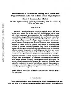
Y’ Figure 1: Transformation from the Cartesian coordinate system (x0; y0; z0), whose (x0; y0; 0) plane lies in the plane of the sky, to the galactocentric coordinate system (x00; y 00; z 00), with the 0x00- and 0y 00 -axes in that plane. The axis of the galactocentric coordinate z 00 is parallel to the z 0 -axis and directed away from the observer. The 0x00 axis coincides with the galactic node line. All coordinate systems are right-handed. The coordinates of the galactic center are (x00; y00 ; 0). The (x00; y00; z00) system is the result of translation of the center of the (x0; y0; z0) system to the center of the galaxy and rotation through an angle �0. The arrow shows the positive direction for rotation of the (x0; y0; z0) system around the z0-axis until it coincides with the (x00; y00; z00) system.
7
Y"
i Y
0
R
B
A
C Vrot
XX" Z"
Z
Figure 2: Transformation from the coordinate system (x00; y00; z00) to the galactocentric coordinate system (x; y; z) with the 0z -axis along the rotation axis for the galactic disk (x; y; z) are galactocentric coordinates, and 0x is the major dynamical semi-axis of the galaxy. The inclination angle i of the galactic plane corresponds to the rotation angle from the sky plane (z00 = 0) to the galactic plane (z = 0). The direction of the line-ofsight coincides with the 0z00-axis. The material point C in the gure is moving away from the observer, i.e., the z00 component of its velocity is positive ((Vrot)z > 0). 00
8
obs Finally, we use a cubic spline passing through the points aobs n (Rl ), bn (Rl ) to deobs obs termine the values for an (R), bn (R) at intermediate points R. This algorithm works well when we have su�ciently good statistical material (beginning with several thousand velocity points evenly covering a ring in the disk containing the spiral structure).
3 Kinematic models for a gaseous galactic disk Since, in observations of galaxies, we can determine only the velocity of gas along the line of sight (from the Doppler shift of lines), i.e., we can measure only one velocity component, we must use some model for the velocity of gas in the galaxy to reconstruct the total velocity. It is natural to consider a number of possible models with varying degrees of complexity, successively including various dynamical factors acting in the galaxy. The crudest of these includes only circular motions, while the most re ned and detailed take account into density waves, the appearance of non-linear harmonics, local small-scale deviations from circular motion associated with star formation, etc. Comparing the Fourier spectrum for the radial velocity predicted by a given model with the observed spectrum allows us to uncover the origin of certain harmonics in the spectrum and to determine the intensity of the action of each dynamical factor in the given galaxy. When the model and observed spectra agree to within the measurement errors, we consider the full velocity eld predicted by the model to coincide with the real velocity eld in the galaxy. As noted in the previous section, even the best modern data permit us to reliably determine only a modest number of coe�cients for the Fourier series of the observed radial velocity. It is evident that these coe�cients determine the most general (but also the most fundamental) characteristics of the velocity eld. In this section, we will attempt to understand the appearance of various Fourier harmonics in the observed radial velocities using two models: a simple model taking into account only circular gas motions (Section 3.1) and a more complex model allowing for the motion of gas in spiral arms (Section 3.2). 3.1. A Simple Model for Purely Circular Motion It is clear that the zeroth and rst harmonics already appear in a simple model with purely circular motion of gas in the galactic disk, where the observed radial velocity is represented in the form (see formula (A4) in Appendix A and Fig. 3)
V mod1(R; ') = Vs + Vrot(R) cos ' sin i; (5) where Vs is the systematic velocity of the galaxy along the line of sight and Vrot is the circular velocity of the gas in the galactic plane, which depends only on the distance from the galactic center { the radius R. If there are only circular motions in the galactic disk, this formula is satis ed with accuracy to the small parameter R/L, where L is the distance to the galaxy. Higher harmonics in the Fourier series can be interpreted using a more complex model, such as the one we will now consider.
3.2. A Model Allowing for Gas Motion in Spiral Arms 3.2.1. General case (arbitrary number of arms). The currently available observations [39, 40] con rm the existence of large-scale systematic deviations from circular motion exceeding the measurement errors. For spiral
9
Figure 3: Derivation of the expression for V mod1 for case i = �=2. It is clear from the gure that ((Vrot)z = Vrot cos '. For the case of arbitrary i, the projection of the trajectory depicted in Fig.2 on the (x00; z00) plane renders (Vrot)z ) = Vrot cos ' sin i. 00
00
10
galaxies, it is most natural to connect these deviations with motions caused by density waves [27, 31, 41, 42]. We therefore propose to consider a speci c model in which the three-dimensional velocity eld in the gaseous disk of a spiral galaxy is associated with a spiral pattern with a particular geometry. Starting from there, a next approximation might be a representation of the radial velocity in the form [see Fig. 4 and formula (A5) in Appendix A, which describes the general case, in contrast to formula (6), where the velocity components are assumed to be associated with the presence of spiral arms; this is the origin of the di�erence in notation for the left-hand sides of formulas (A5) and (6)] (6)): V mod2(R; ') = Vs + Vr (R; ') sin ' sin i + V'(R; ') cos ' sin i + Vz (R; ') cos i ; (6) where
Vr (R; ') = V~r (R; ') ; V'(R; ') = Vrot(R) + V~' (R; ') ; Vz (R; ') = V~z (R; ') : (7) Here Vr , V' , Vz are the components of the galactocentric velocity in the gaseous disk, and V~r , V~', V~z are the components for the velocity of the motions associated with the density wave. In the case of purely circular motion (Vr = 0, V' = Vrot(R), Vz = 0), formula (6) obviously reduces to formula (5). Account of the last term in (6), containing Vz is one of the principle di�erences of the method proposed here from those used earlier. This term is essential, since in addition to motions in the disk plane, the density wave creates vertical motions that can be neglected only in very rare special cases [43]8. A natural general approach to relating the characteristics of the observed radial velocity eld to motions in a density wave is Fourier analysis of the observations using expression (6). Expanding the velocity deviations on the right-hand side of (6) caused by the spiral in a Fourier series and equating these model coe�cients to the observed coe�cients for the corresponding harmonics in equation (1), we can obtain a set of equations that can be used to calculate the full three-dimensional velocity eld of the galactic gas. However, this problem is di�cult to solve in such a general formulation. Here, we are concerned with an analysis for the case of galaxies with a fully determined number of arms m. The preferential development of spiral structures with a well-de ned number of arms could have various origins: the presence of a maximum instability increment corresponding to the mode m, or the growth of perturbations exclusively with mode m, when the development of other modes is suppressed for some reason. For example, the development of the mode m = 2 could be facilitated by a tidal interaction with a neighboring galaxy and/or the preferential development of bar-mode instabilities, etc. (for more detail, see [47]). In this case, we expect that the component with azimuthal number m will be most strongly represented in the residual velocity eld. This As we will see below, the only perturbations determining the mth harmonic of the observed radial velocity for an m-arm galaxy are perturbations in Vz . Here, we consider only motions along the disk rotational axis that are associated with density waves { spiral arms. These correspond to antisymmetric perturbations V~z , relative to the plane z = 0. Symmetric perturbations V~z describe "bending" oscillations [44], which may be caused by " rehose" instabilities [44-48]. Such perturbations are considered in detail in [47]. 8
11
Figure 4: Derivation of the expression for V obs . As in Fig. 3, the case i = �=2 is considered. However, in contrast to Fig. 3, the material point C rotates does not move only in a circular trajectory, but rather participates in three simultaneous motion in R, ', and Z . Thus, contributions to the radial velocity are made by the projection onto the z00-axis (VR)z = VR sin ', (V' )z = V' cos ', and the z00 component of the systematic velocity. For i = �=2, the Vz component does not contribute. For arbitrary i, we have Vobs = Vs + (VR sin ' + V' cos ') sin i + Vz cos i. 00
00
12
is clearly true for small amplitude ("linear") perturbations. However, even for the case of non-linear perturbations, such as most of the observed spiral arms, the main large-scale mode can have a predominant amplitude, especially in a velocity eld where the residual (perturbed) velocities are much smaller than the circular (unperturbed) velocities, so that in some sense, the condition for the linear approximation is satis ed9. In addition, the presence of other factors giving rise to non-circular motions, such as outbursts of star formation and measurement errors, can strongly a�ect the small-scale components of non-circular velocities and make their interpretation more di�cult. As a result, only galaxies with a clearly-expressed predominance of a fundamental large-scale mode can currently be reliably analyzed using this method. As we will show below, the suitability of each galaxy for analysis using the method described here can be veri ed directly from the character of the observed radial velocity eld. The main advantage to the case with predominance of a fundamental mode is the ease of representing the residual velocities as harmonics and the possibility of using relations between them analogous to those obtained from the hydrodynamic equations in the linear approximation. Below, we will represent the residual velocities in terms of their amplitudes Cr , C' and Cz (all Ci > 0) and phases Fr , F', Fz :
V~r (R; ') = Cr(R) cos[m' ? Fr(R)] ; (8) V~'(R; ') = C'(R) cos[m' ? F'(R)] ; (9) V~z (R; ') = Cz (R) cos[m' ? Fz (R)] : (10) Substituting the equalities (7)-(10) into expression (6) for the radial velocity, we nd that in the framework of our model, taking into account interactions between gaseous clouds and spiral density waves, the radial velocity has the form V mod2(R; ') = Vs + sin i [ Vrot(R) cos '+ + am?1(R) cos(m ? 1)' + bm?1(R) sin(m ? 1)' + + am(R) cos m' + bm(R) sin m' + + am+1(R) cos(m + 1)' + bm+1 (R) sin(m + 1)' ] ; (11) where the coe�cients for the harmonics on the right are the coe�cients of the Fourier expansion of the function V mod2(R; ') in the coordinate '10. These are equal to am?1 = Cr sin Fr +2 C' cos F' ; (12) bm?1 = ? Cr cos Fr ?2 C' sin F' ; (13) am = Cz cos Fz cot i ; (14) bm = Cz sin Fz cot i ; (15) Studies of the galaxies NGC 157 and NGC 6181 using this method [38] showed that the velocities of non-circular motions near the corotation radius caused by the spiral arms are more than a factor of ve smaller than the circular velocities in the disk. 10To avoid unwieldiness, we drop the notation "mod2" for these coe�cients here and below. 9
13
(16) am+1 = ? Cr sin Fr ?2 C' cos F' ; bm+1 = Cr cos Fr +2 C' sin F' : (17) The remaining coe�cients of the Fourier expansion of V mod2 are equal to zero. It is clear from these relations that the contributions of the velocity components of the galactic gas to the azimuthal Fourier harmonics of the observed radial velocities are as follows:
� The systematic velocity of the galaxy contributes to the zeroth harmonic, � Purely circular motion contributes to the cosine coe�cient of the rst harmonic. � The mth harmonics of the galactocentric radial and azimuthal velocities in the galactic plane contribute to the (m ? 1)th and (m + 1)th harmonics. � The mth harmonic of the vertical velocity contributes to the mth harmonic. Thus, if a galaxy has m spiral arms, the (m ? 1)th, mth, and (m + 1)th harmonics
should be present in the velocity eld observed along the line of sight, along with the zeroth and rst harmonics. Note that since formulas (8)-(10) are approximations, this conclusion is valid only for galaxies with a clearly-expressed predominance of a fundamental harmonic in the velocity eld. On the other hand, observational veri cation of this conclusion makes it possible to determine the correctness of representing the residual velocities in the form (8)-(10). If the signi cant harmonics are the zeroth, rst, (m ? 1)th, mth, and (m + 1)th, then this forms a basis for using the model speci ed here. It follows that in analyzing the Fourier spectrum of the observed radial velocity eld, we can obtain in a self-consistent way the coe�cients for the zeroth harmonic specifying the systematic velocity of the galaxy as a whole, the cosine of the rst harmonic enabling calculation of the galactic rotation curve, and the (m?1)th, mth, and (m+1)th harmonics determining non-circular motions caused by the density wave. 3.2.2. The case of many-armed spirals (m � 3) and a Fourier series of ve harmonics. Let us suppose that we have deterrnined the main parameters specifying the position of the galactic plane using independent methods: its inclination angle, its position angle, and the position of its rotation center. In this case, if the galaxy is many-armed (m � 3), it is possible to determine all three components of the gas velocity at any point of the galactic disk using only the assumptions made earlier. In fact, in this case, Vs , is the zeroth harmonic and Vrot is the cosine coe�cient of the rst harmonic. We further nd from the observations the additional six coe�cients am?1, am, am+1, bm?1 , bm, bm+1 associated with the six equations (12)-(17) in the six unknowns Cr , Fr , C', F', Cz , Fz , which fully determine motions in the spiral arms. Thus, in general, for m � 3, we nd from the observations eight Fourier coe�cients for eight unknown functions. 3.2.3. The degenerate case of two-armed spirals (m = 2) and a Fourier series of four harmonics.
14
The case of two-armed spirals (m = 2) is an important exception. In this case, the cosine coe�cient of the rst harmonic simultaneously contains contributions from circular motion and from motion caused by the density wave:
aobs (18) 1 (R) = Vrot (R) + a1 (R) ; where a1 is given by expression (12). As a result, the system of equations (l 1) { (17) becomes undetermined11. Directly from radial velocity observations, we can determine only the systematic velocity of the galaxy Vs and the amplitude Cz and phase Fz characterizing the vertical obs motions caused by the spiral wave. Knowledge of the four additional quantities aobs 1 , a3 , obs obs b1 ¨ b3 allows us to obtain the four equations (for each speci c galactocentric radius) Vrot + Cr sin Fr +2 C' cos F' = aobs (19) 1 ; ? Cr cos Fr + C' sin F' = 2 bobs (20) 1 ; ? Cr sin Fr + C' cos F' = 2 aobs (21) 3 ; Cr cos Fr + C' sin F' = 2 bobs (22) 3 ; containing the ve unknowns Vrot , Cr , Fr , C' ¨ F'. Consequently, in order to determine
the rotation curve and reconstruct the full velocity eld for two-armed spiral galaxies, we must use an additional equation. Below, we consider three di�erent ways to obtain an additional condition for the unknown functions. In the rst case, this condition is a relation between the phases of velocity components, and in the second, it is a relation between the phases of the radial velocity component and the surface density. In the third case, we use a condition essentially replacing the missing fth equation. Method 1, relations between phases of the radial and azimuthal velocities. From the linearized system of three-dimensional hydrodynamical equations for a compressed barytropic rotating medium, we obtain for the residual radial and azimuthal velocities (see, for example, [43])
v~r = ?i^!�~ +D2mi ~�=R ; (23) 0 2 (24) v~' = ?�~ � =2 D+ m!^ �~=R : Here, we have used a complex representation of the perturbations in the form exp[i(m' ? !t)], !^ � ! ? m is the frequency of the wave in a comoving reference system (at the corotation radius, !^ = 0), � Vrot=R is the angular velocity of the disk rotation (as shown by Poincare, this is constant throughout the thickness of the disk); D � !^ 2 ? �2, � is the epicyclic frequency (�2 � 2 (2 + R 0)), a prime denotes di�erentiation in radius; i is the square root of (-1); and �~ is the potential of the perturbing force (i.e., the force giving rise to the deviations in the velocity from circular). This force can 0
In particular, it follows from this that, even in the presence of an arbitrarily detailed radial velocity eld, the rotation curve determined using a model with purely circular motion will have systematic errors; as follows from (18), these will be larger the higher the velocity in the spiral wave. 11
15
include self-gravitation of the disk, pressure, the external action of the stellar disk, a bar, or a companion, etc. Relations (23) and (24) should be understood as in reality equating the real parts of the expressions on the left- and right-hand sides. The physical perturbed velocities can be obtained from the complex velocities determined by relations (23) and (24) by taking their real parts. For example,
U~r = Ar cos(m' ? �r ) = Re(~vr ) ; (25) whence u~r = Ar exp(i m' ? i �r ), etc. The di�erence between the amplitudes and phases in relations of the form (25) and the amplitudes and phases of the velocity components determining the model radial velocity eld (6) and entering relations (8)-(10) is that the former may depend on the coordinate z perpendicular to the disk. The radial velocity eld, which is dependent only on the coordinates R and (p in the plane of the disk, is the result of averaging over the line of sight. This is a1so true for the velocity components (8)-(10) entering the model expression (6). In contrast to the perturbed velocities U~r , U~', U~z we will term the velocity components V~r , V~', V~z "residual." Because of the small thickness of the disk, the averaging along the line of sight can be represented as an integration perpendicular to the disk with some weight that depends on the observing conditions. For example, in the space between the arms, the optical depth of the disk is small: there, the weakening of the light by dust is several tenths of a magnitude [49]; the "weight" is therefore close to the function �(r; '; z), i.e.12, +1 r; '; z )U~ (r; '; z )dz ? V~? (R; ') = ?1 �(+1 ; (26) � ( r; '; z)dz ?1 where the notation ? indicates any component of the residual velocity parallel to the plane of the disk (perpendicular to the z-axis). The optical depth t of the spiral arms can be substantially di�erent between and in stellar complexes [50]. If � � 1 at the half-thickness of the disk between complexes, then in a stellar complex, optical depths � � 1 are encountered several tens of parsecs before reaching the plane z = 0 [49]. In this case, we can approximately take the residual velocity V~? (r; ') to be the result of averaging the velocity perturbations U~?(r; '; z) over the half of the disk thickness turned toward the observer, as before with weight close to �(r; '; z)13. Below, we will consider relations between the phases of the radial and azimuthal residual velocity components. If we knew the "weight" for averaging along the line of sight and the dependence of the velocity perturbations on z, it would not be di�cult to obtain these relations. However, as a rule, neither the rst nor the second quantity is known, and it is a separate, complex task to derive the connection between the velocity R
R
In this formula, the function � denotes the total and not the perturbed volume density of the gas, whose emission intensity is taken to be proportional to �. 13Note that precisely the presence of a region with � � 1 makes it possible to observe the vertical component of the perturbed velocity. Otherwise, due to the fact that v~z (z) is an odd function, there would be a mutual cancelling of contributions for regions with vertical velocities with opposite sign during the averaging across the disk, and the averaged value would be close to zero. 12
16
perturbations and the residual velocities. We therefore carry out our analysis for cases when it is possible to unambiguously relate at least the phases of these two velocities. First, this can be done at the corotation radius, where the velocity perturbations, and consequently their phases, do not depend on z. This follows from the equation of motion for the z coordinate [43]: i^!v~z = @ �~=@z : (27) For corotation, !^ = 0 and the function �~ does not depend on z. Consequently, according to (23), (24), and the result of Poincare noted above, the functions v~r and v~' also do not depend on Z 14. Second, if the relation between the phases of the perturbed velocity components do not depend on z, the same relation will be satis ed for the phases of the residual velocities. Essentially, the rst of these possibilities is a special case of the second. Let us consider how to obtain a relation for the phases of the perturbed velocities that is independent of z. We obtain from expressions (23) and (24) the relation between the radial and azimuthal perturbed velocities: v~r = i^!�~0 ? 2mi ~�=R : (28) v~' �~0�2=2 ? m!^ �~=R For most observed spirals, the "tightly-wound spiral" condition
jkr jR � m ; (29) is well satis ed; here, jkr j = j(ln f~)0j ' 2�=� is the radial wave number, which, generally speaking, can be complex15; f~ is any perturbed function (for example, �~, v~r or v~'); and � is the wavelength of the spiral pattern. Note that the strong inequality (29) does not precisely correspond to the name we have given this condition: it is ful lled even for open (R=� ' 1), one-armed (m = 1) spirals, and is ful lled for two-armed spirals (m = 2) with R=� > 3, also not corresponding to tight winding. Condition (29) is ful lled with 30% accuracy for open two-armed spirals. We also note that the approximation (29) is substantially softer than the WKB approximation, since the latter requires not only that the wave number be large, but also that it vary slowly in radius. Using the representation for �~ in the form of a spiral [51],
�~(R; '; t) � exp[i(
Z
R
kr dr + m' ? !t)]:
(30)
Strictly speaking, this argument is not entirely correct, since the perturbed velocities depend not only on �~, but also on its radial derivative. This derivative may depend on z, despite the constancy ot the function itself in the vertical direction at the corotation radius. Nonetheless, since in the vicinity of the corotation radius for small !^ the dependence of �~ on z will also be small, we expect that the dependence of the radial derivatives on z will be signi cant only to higher order. An accurate analysis con rms these simple notions, and shows that variations in the perturbed velocities perpendicular to the disk appear only to next order in the approximation of a tightly-wound spiral. Therefore, all the reasoning presented here and further, in Section 4.3, are valid with accuracy to terms of the order of 1=(jkr jR). 15Below, we assume that jImk j � jRek j. This inequality corresponds well to the observations: over r r a signi cant extent on either side of the corotation radius, the arm brightness does not vary as much as it would if this inequality were not ful lled. 14
17
and condition (29), the relation between the radial and azimuthal perturbed velocities (28) can be appreciably simpli ed: v~r � i2 ^! ? 4m 2 : (31) v~' �2 kr R�2 When deriving (31), we omitted the second term in the denominator of (28), using the condition of tight winding. However, we can not, generally speaking, neglect the second term in the numerator of (28), since the rst term is proportional to !^ , which is small near the corotation radius. Since v~r =v~' = (Ar =A') exp[i(�' ? �r )], relation (31) is most easily used to obtain the relation between the phases of the radial and azimuthal perturbed velocities. In this case, we do not need to know the exact values of the parameters for the wave and disk appearing in (31), but only their signs. These signs depend on the direction of rotation of the disk in the plane of the sky, the type of spiral, and the choice of sign for the azimuthal number m. Therefore, in order to ensure an unambiguous treatment of the phase relations obtained below, we formulate several initial premises. (1) The galaxies considered have trailing spirals. This assumption is important for correct choice of the inclination angle of the galaxy and correct sign for its rotational velocity. It was convincingly shown [52] using a large set of observational material (190 spiral galaxies) that in all cases when the galaxy can be taken to be an isolated (conservative) system, its spiral arms are trailing. Of the 190 galaxies indicated in [52], 19 can not be considered isolated; in three of these, the spirals are leading. Fridman has suggested that a su�cient condition for the generation of leading spirals in a galaxy is the presence of a close companion with its orbital moment opposite to the rotational moment ("spin") of the main galaxy. Indeed, all three galaxies with leading spirals have close companions, however it was possible to measure the direction of the orbital moment of the companion relative to the "spin" of the main galaxy for only one of these. In this one case, the moments proved to be oppositely directed. In laboratory experiments with rotating shallow water [18], the main conditions for forming leading spirals with a close "counter-rotating" companion were produced, and leading spiral density waves were obtained. The analysis for gaseous disks with exotic leading two-armed spirals is entirely analogous to the analysis for trailing spirals presented below, with account for the sign change of the wave number kr . (2) In the coordinate system of the observer, the directions of the phase velocity of rotation of the spiral and of the angular velocity of rotation of the disk coincide, and the relation between their absolute values indicates that the corotation radius Rc is less than the disk radius Rd , i.e., Rc < Rd. This premise a�ects the sign of !^ and is satis ed for all known cases when the reason for excitation of the spiral wave is associated with the disk itself. As we will show in Section 4, the presence of a corotation region and the sign of !^ can be veri ed directly from observations. Therefore, this premise is presented mostly for clarity and simplicity. (3) The azimuthal number m is always positive, m > 0, i.e., it always coincides with the number of arms. Arbitrariness in the choice of sign for the azimuthal number is a consequence of the complex representation for physical quantities used in the physics literature, and does not 18
a�ect the nal result. In our case, reconstruction of the velocity eld does not depend on a priori choice of the sign for m. This premise is required only in order to prevent incorrect treatment of the inter- mediate results presented below. (4) A right-hand coordinate system is used. The comments for the previous premise are entirely relevant for this assertion as well. Let us consider in sequence the two possible directions of rotation of the galactic disk in the plane of the sky. (A) The direction of rotation of the disk is positive ( > 0), i.e., it coincides with the direction of increasing angle '. In this case, due to premise (2), the phase velocity of the wave is positive, i.e., !ph � !=m > 0, and due to premise (3), we have ! > 0. In all cases known to us, the angular velocity falls with radius. Therefore, if > 0 before corotation, !^ < 0, and after corotation, !^ < 0. The sign of kr is determined by the shape of the spiral. On the line of constant phase m' + kr dR = const. It follows that along this line, dR=d' = ?m=kr . If the rotational velocity is positive, a trailing spiral will wind to the right as it moves from the center. Consequent1y, for such a spiral, kr > 0 (Fig. 5a). (B) The direction of rotation of the disk is negative ( < 0). In this case, due to premise (2), the phase velocity of the wave is negative !ph < 0, and we therefore have ! < 0. Analogous to case (A), we nd that for < 0 before corotation, !^ > 0 and afterwards !^ < 0. For a negative rotational velocity, a trailing spiral will wind to the left as it moves from the center. Consequently, in the case considered, kr < 0 for a trailing spiral (Fig. 5b). The resulting signs for the main parameters of the disk and spiral structure are presented in the rst line of the table. Using these data, we nd from (31) v~r = � i2j ^!j ? 4m 2 ; for > 0; (32) v~' �2 jkr jR�2 and v~r � � i2j ^!j + 4m 2 ; for < 0 : (33) v~' �2 jkr jR�2 Here and below, the upper sign corresponds to the region before corotation (R < Rc) and the lower sign to the region after corotation (R > Rc ). The phase relations at some distance from the corotation radius. Far from the corotation radius, the absolute values of the second terms in (32) and (33) are small compared to the rst terms by a factor � (jkr jR)?1, and they may be omitted. Consequently, beyond the corotation region, the relation between the phases for the radial and azimuthal perturbed velocities does not depend on the direction of the disk rotation, but does depend on the sign of �2, i.e., on the degree of di�erential rotation16. R
Recall that, if absolute values of the rotational velocity fall with radius as j j � R?� , the square ot the epicyclic frequency becomes negative, � > 2. This case is encountered among galaxies extremely rarely { the only example known to us is Mkr 1040 [32]. The speci c character of this rotation law is 16
19
Figure 5: Determination of the sign of kr . In the right-handed coordinate system used, the 0z axis is directed away from the observer and the azimuthal angle increases in the clockwise direction. The direction of the rotation corresponding to increasing ' is positive. (a) A trailing spiral for > 0. It is clear that dR > 0 for d' > 0. Consequently, the spiral equation dR=d' = ?m=kr is satis ed for kr > 0. (b) A trailing spiral for < 0. It is clear that dr > 0 for d' > 0. Consequently, the spiral equation is satis ed for kr < 0. It follows that, for trailing spiral, the sign of the radial wave number kr coincides with the sign of .
20
For �2 > 0, we obtain17 and for �2 < 0
�'(R) = �r (R) � �=2 ;
(34)
�'(R) = �r (R) � �=2 : (35) The resulting relations are universal in the sense that they do not depend on the nature or type of perturbing potential [far from the corotation region, the derivatives vanish from the denominator and numerator of (28)]. In particular, they do not depend on representation of �~0 in the form (30) or on the form of the wave number k", which can be an arbitrary complex number that varies arbitrarily rapidly. Another important consequence of this universality is that the relations between the phases for the velocity components are constant over the entire thickness of the disk. As a result, as we showed above, these relations are valid both for local perturbed velocity components and for residual velocities averaged (with some weight) over the disk thickness. Finally, for the phases Fr , and F' in relations (8) and (9), we have (Fig. 6)
F'(R) = Fr (R) � �=2 ; for �2 > 0 ; (36) F'(R) = Fr (R) � �=2 ; for �2 < 0 : (37) The resulting expressions show that there is a change in the relation between the velocity component phases in some region near the corotation radius. In order to use expressions (36) and (37), we must therefore determine (from observations) the corotation radius and the width of the region over which the phase relations change. Since it is also necessary to determine the corotation radius in order to nd the rotational velocity of the spiral-vortex structure, which is a problem of fundamental importance, we will consider these issues separately in Section 4. Another di�culty in using (36) and (37) is phase ambiguities. For example, in (36), for equivalent (i.e., to within 2�) phase di�erences before the corotation radius, the change in the phase relation in the corotation region can be either a continuous decrease in the phase di�erence from 3�=2 to �=2 or a continuous increase from ?�=2 to �=2.
The phase relations at the corotation radius. In order to exclude the indicated phase ambiguity, it is su�cient to determine the phase di�erence at the corotation radius. Here, the rst terms in (32) and (33) vanish, so that for �2 > 0 we have
and for �2 < 0
F'(Rc) = Fr (Rc) + � ;
(38)
F'(Rc) = Fr (Rc) :
(39)
such that, in both the hydrodynamics of incompressible uids (between two rotating cylinders [53]) and in stellar dynamics [54], it is unstable. 17When using the phase relations presented below, it is important to remember that they are determined only with accuracy to 2�.
21
Here have accounted for the fact that the phases � and F coincide at the corotation radius. Expressions for the amplitudes and phases of the three velocity components. The additional conditions provided by the phase relation for the radial and azimuthal residual velocities together with equations (19)-(22) make up a closed system of equations. Using relation (36) as an example, we will show how this makes it possible to determine the full vector velocity eld, i.e., the amplitudes and phases of all three velocity components. Substituting conditions (36) brings the system of equations (19)-(22) into the form 1 Vrot = aobs (40) 1 ? 2 (Cr � C' ) sin Fr ; (Cr � C') cos Fr = ? 2 bobs (41) 1 ; (Cr � C') sin Fr = ? 2 aobs (42) 3 ; (Cr � C') cos Fr = 2 bobs (43) 3 : We now easily obtain for the amplitudes and phases of the radial and azimuthal residual velocity components and for the rotational velocity the expressions obs tan Fr = ? cot F' = ? aobs (44) 3 =b3 ; (bobs 3 )2 obs (45) cos Fr = sign bobs ? b 3 1 obs ; (aobs 3 )2 + (b3 )2 obs Cr = (bobs (46) 3 ? b1 )= cos Fr ; obs C' = � (bobs (47) 3 + b1 )= cos Fr ; obs bobs a obs (48) Vrot = a1 ? 3bobs1 : 3 Expressions for the amplitude Cz , and phase Fz , of the vertical velocity component can be found from equations (14) and (15). Thus, these formulas make it possible to reconstruct the vector velocity eld of the gaseous disk of a spiral galaxy from the coe�cients of the Fourier expansion of the observed radial velocities. Method 2, relations between the phases for the radial velocity and perturbed density18. Another way to close system (19)-(22) is to use information about the density distribution in the spiral wave, obtained from photometric data, and the relation between the characteristics of the density and residual velocities, following from density wave theory. When deriving the necessary relations, we will use the continuity equation, which in the linear approximation has the form @ � v ~ (49) !^ �~ = ? Ri (R�v~r )0 + m ' ? i (�v~z ) ; R @z v u �u t
�
18To use these relations, we must know F (R). This quantity determines the shape of the spiral, and � can therefore be found from observations, for example, from Fourier analysis of the brightness distribution of the galaxy, as shown in [55].
22
where � and �~ are, respectively, the unperturbed and perturbed volume gas density in the disk. Integrating this continuity equation over z, we obtain +1 +1 !^ �~ = ? Ri (R�v~r )0 dz + m (50) R ?1 (�v~')dz: ?1 +1 �~dz , the Here, we have used the de nition of the perturbed surface density �~ = ?1 condition for the absence of matter at �1, and the lack of dependence of the angular velocity of rotation on z. In the small pitch angle approximation (29), equation (50) simpli es and takes the form Z
Z
R
Z
+1
(�v~r)0 dz; (51) !^ �~ = ? i ?1 and to calculate this integral, we must know how the functions � and v~r , depend on z, which, generally speaking, we do not. However, in the two regions of the gaseous disk considered earlier | between the spiral arms (where the disk can be considered optically thin) and in the arms (where only the nearest half-thickness of the disk can be considered optically thin) | we can relate the right-hand side of (51) with the radial residual velocity component V~r . Using expression (26) for both cases (in the second case, the integration is taken from 0 and not from ?1, and we must take account of the fact that the radial velocity perturbations in the density wave are even functions of z), we obtain +1 �(R; ?1
Z
'; z)U~r (R; '; z)dz = �(R; ')V~r (R; ') :
(52)
As a result, (51) is transformed to the form
�~ =� = kr V~r =!^ :
(53)
The phase relations at some distance from the corotation radius. As before, assuming jIm kj � jRe kj and using the rst line of the table we nd that, for both > 0 and < 0, the ratio �~ =V~r , is equal to
�~ =V~r = ��jkr=!^ j : (54) From this, we nd the relation between the density and radial velocity phases (Fig. 7): Fr (R) = F� (R) + �; for R < Rc; (55) Fr (R) = F� (R); for R > Rc: The linearized continuity equation used in our derivation of (55) can not be considered completely correct, since �~ =� > 1 in spiral arms. In spite of this "seditious" comment, we nonetheless wish to maintain that conditions (55) are valid. The reason for this is very simple: numerical experiments using non-linear hydrodynamic equations (see, for example, [26]) show that the phase of a spiral density wave whose amplitude grows is virtually constant. This means that, having determined relations (55) for small values �~ =� � 1, when the linearized continuity equation is clearly valid, we should not observe signi cant variations in (55) with growth in the ratio �~ =�. 23
Figure 6: Di�erence in phase of the azimuthal and radial velocity components as a function of radius. The solid lines correspond to the case > 0 and the dashed lines to the case
< 0. (a) �2 > 0; the angular velocity of rotation of the disk falls with radius more smoothly than R?2 . (b) �2 < 0; the angular velocity of rotation of the disk falls with radius more sharply than R?2 .
Figure 7: Same as Fig. 6 but for the di�erence in phase of the radial velocity and surface density. 24
At the same time, relations (55) make it possible to use independent photometric information, and in this sense enhance the reliability of our results; when the velocity elds reconstructed using our rst two methods agree, relations (55) demonstrate the relation between the observed residual velocities and the density wave. The di�culties in using (55) are the same as those for (36) and (37). The biggest of these is that relation (53), from which (55) follows, is not satis ed in the direct vicinity of the corotation radius, where the denominator of the right-hand side of (53) becomes very small. We estimate the size of the region where the relation (55) between the phases becomes invalid in Section 4. A second di�culty is, again, caused by phase ambiguity, and it is therefore necessary to determine the phase di�erence at the corotation radius. The phase relations at the corotation radius. Let us write an expression for the velocity v~r , at the corotation radius: m �~ = ? i 2m c2 �~ + �~ : v~r = i 2RD (56) R�2 � Here, �~ is the perturbation of the gravitational potential, and we have used the expression for D at the corotation radius D = ?�2, as well as the de nition � � c2�~=� + �~ [43]. Multiplying (56) by � and integrating over z from ?1 to +1, we obtain m c�2�~ + � ~ ; v~r � = ? i 2R� (57) 2 where we have taken into account the fact that v~r does not depend on z at the corotation radius (see above) and, following [43], have introduced the notation !
�
c�2 � �~ ?1
+1 2 c �~dz ; ?1
Z
~ � �?1
�
Z
+1
?1
��~ dz :
(58)
Using also the simple local relation between ~ and �~ [43], ~ = ? 2�G�~ ; (59) jkj we obtain from (57) v~r = i 2m : (60) �~ �2R� When deriving (60), we used the dispersion equation [43], which at the corotation radius has the form
�2 ? 2�G�0jkj + k2c�2 = 0 : (61) Using the rst line of the table and taking into account the equality of the phases of the perturbed and residual velocities at the corotation radius, we obtain (Fig. 7) from (60) for �2 > 0 and for �2 < 0
Fr (Rc) = F� (Rc ) ? �=2 ; 25
(62)
Fr(Rc ) = F� (Rc) + �=2 :
(63)
Expressions for the amplitude and phase of the three velocity components. The additional condition (55) { the relation of the phases of the density and radial residual velocity { together with equations (19) { (22) permit us to determine the full vector velocity eld, i.e., the amplitudes and phases of all three velocity components. Using condition (55), i.e., taking Fr to be unknown, we obtain from system (l9) { (22) obs obs (64) Cr = � b3cos?Fb1 ; � obs ? bobs ) tan F obs � 1 3 ; (65) cot F' = 2a3 + (bbobs obs 3 + b1 obs 2 obs obs obs 2 1=2 C' = f(bobs (66) 3 + b1 ) + [2a3 + (b3 ? b1 ) tan F� ] g ; obs sin F' = (bobs (67) 1 + b3 )=C' ; obs obs obs Vrot = aobs (68) 1 ? a3 ? (b3 ? b1 ) tg F� : As above, the upper sign corresponds to the region before corotation and the lower sign to the region after corotation. Method 3, valid when the amplitudes Cr , and Cz depend weakly on radius. To reconstruct the velocity eld using relations (19) { (22) independent of any density wave model, we can use the assumption that all observed functions vary smoothly. Since, according to relations (20) and (22), obs Cr cos Fr = bobs (69) 3 ? b1 ; obs C' sin F' = bobs (70) 3 + b1 ; we expect that when the amplitudes Cr and C' depend only weakly on radius (i.e., the density wave pro le is smooth), the locations of the extrema of the observed quantitites on the right-hand sides of (69) and (70) will be close to the positions with corresponding phases for the radial and azimuthal velocities. Accordingly, the values for the right-hand sides at the extremal points specify the amplitudes of the residual velocities in these sections of the disk. This makes it possible to nd all the desired quantities. obs Supposing that bobs 3 ? b1 achieves an extreme value at radius R, taking into account the above discussion we nd that at this radius, obs Fr = �=2 ? sign(bobs (71) 3 ? b1 )�=2 ; obs (72) Cr = jbobs 3 ? b1 j : From these last two formulas and formulas (19) { (22), we nd at this same radius the remaining desired quantities:
C' =
q
obs obs (2aobs 3 )2 + (b3 + b1 )2 ;
26
(73)
obs obs obs sin F' = b3 C+ b1 ; cos F' = 2Ca3 ; ' ' obs obs Vrot = a1 ? a3 : obs Supposing now that bobs 3 + b1 achieves an extreme value at radius R, we have
(74) (75)
obs F' = sign(bobs (76) 3 + b1 )�=2 ; obs C' = jbobs (77) 3 + b1 j : From these last two formulas and formulas (19) { (22), we obtain at this same radius q
obs obs Cr = (2aobs (78) 3 )2 + (b3 ? b1 )2 ; obs obs obs sin Fr = ? 2aC3 ; (79) cos Fr = ? b3 C? b1 ; r r obs Vrot = aobs (80) 1 ? a3 : This method makes it possible to independently verify the correctness of the velocity reconstruction for the rst two methods at extremal points. Assuming that Vrot(R), Cr (R), and C'(R) are smooth functions, we can in each of the methods described also reconstruct the values for all the desired functions at intermediate points (in the simplest case, by linear interpolation of Vrot(R), Cr (R), and C'(R)). Each of the methods described for the reconstruction of the velocity eld has its shortcomings; however, we expect that using them together will make it possible to avoid systematic errors and obtain a model for the galactic velocities that is close to the real situation. Agreement of the results for the three independent methods to within the observational errors can serve as evidence of the correctness of the velocity eld reconstruction.
4 Finding the corotation radius of the spiral-vortex structure Finding the corotation radius R, in spiral galaxies is one of the most important problems in this eld. A number of methods for determining this radius are described in the literature, however they often lead to di�erent results. Most of these methods use the observed shape of the spiral arms, brightness distribution of the disk, and rotation curve. Further, the surface density distribution and velocity dispersion in the disk are found, with the constraint that these functions be consistent with the selected disk model and correspond to the shape of the density wave. This density wave is derived from wellde ned concepts about its nature and should coincide with the observed spiral pattern. The aggregate of model-dependent ideas and free parameters (for example, choice of the azimuthal phase velocity for the density wave) that characterize these models are not a point in their favor. In this section, we describe three independent methods for determining the corotation radius, using only observational data and a fundamental hypothesis: the spiral 27
pattern is a density wave. If we exclude this last assumption, we lose the very concept of a corotation radius where the constant angular velocity of the spiral pattern coincides with the velocity of the di�erentially rotating galactic disk. Any other (nonwave) structure will be disrupted by the di�erential rotation (recall non-linear tidal waves that move along the complex channels of rivers and canals virtually without changing their shape and velocity [56]). Based on the analysis in Section 3, we conclude that the corotation region is characterized by variations of certain relations between the phases of separate density wave parameters, which preserve their appearance at all other places in the disk. Consequently, in order to localize the corotation radius, we must nd the region where relations (36) for (37) for �2 < 0] and (55) break down. We will show how this can be done using the obs obs obs observed radial velocity eld, i.e., knowing the coe�cients aobs 1 , b 1 , a3 ¨ b 3 . 4.1. The First Method for Finding the Corotation Radius In order to obtain an observational criterion for the change of sign of the phase di�erence for the radial and azimuthal residual velocities, note that taking into account the strict positivity of the amplitudes Cr , and C', the conditions obs jbobs 3 (R)j ? jb1 (R)j � 0; for R < Rc ; obs jbobs 3 (R)j ? jb1 (R)j � 0; for R > Rc
(81)
j!^ �~0j � j2m ~�=Rj :
(82)
follow from expressions (46) and (47). It follows from these inequalities that the corotation obs radius should be located in the region where jbobs 3 (R)j ? jb1 (R)j changes sign. Let us estimate the size of the corotation region that can be expected using criterion (81). First, we will elucidate at what distance from the corotation radius the phase relation (36) begins to be valid. When deriving this relation, we used the inequality (in the small pitch angle approximation) Accordingly, relations (36) will vary in the region where
j!^ j ' 2m R�~�~0 : (83) Expanding the left-hand side in a series near the corotation radius and assuming a nearly at rotation curve � 1=R, we estimate for the size of the corotation region, outside of which we can use relation (36):
j�Rj ' j2=kj :
(84)
We can obtain an estimate from above using the global spiral wavelength in radius. In this case, the restriction to (84) yields j�Rj � � ' 0:3 : (85) R �R Thus, the phase relations (36) can be considered valid at a distance from the corotation radius of about 1/3 this radius. 28
4.2. The Second Method for Finding the Corotation Radius A somewhat di�erent method for determining the corotation radius can be derived from expressions (64), taking into account the strict positivity of the amplitude Cr : obs (bobs 3 (R) ? b1 (R)) cos F� (R) � 0; for R < Rc ; (86) obs (bobs 3 (R) ? b1 (R)) cos F� (R) � 0; for R > Rc : It follows from these inequalities that the corotation radius should be located in the region obs where (bobs 3 ? b1 ) cos F� changes sign. Let us estimate the restriction on the location of the corotation radius imposed by criteria (86). We expect that relation (55) between the phases of the radial velocity and density, which was used with expression (64) to derive (86), will be approximately true if two conditions are satis ed:
jkv~r j � jmv~'=Rj ; j�~=�j ' jkv~r=!^ j � 1 :
(87) (88) The rst condition corresponds to neglecting the azimuthal residual velocities in the continuity equation. The second condition delimits the region where ful llment of relation (53) does not require strong non-linearity. Using relation (31) between the residual velocities in the region of small pitch angle of the spiral and expanding !^ in a series near the corotation radius [analogous to the derivation of (84)], we nd that condition (55) makes it possible to delimit the corotation region with accuracy to v~r ; j�Rj ' max k1 ; R kR (89) m Vrot where the rst factor on the right-hand side appears due to (87) and the second factor appears due to (88). Comparing with our estimate of the corotation region using the phase relation for the azimuthal and radial residual velocities (84), we see that our use of information about the phase of the density is attended by an additional condition associated with the nonlinearity of the density. Taking for our estimate � ' R and v~r ' (0:05 � 0:1) Vrot, we nd that the nonlinearity restriction allows us to delimit the corotation region with accuracy not better than j�Rj ' 2�R v~r ' 0:15 � 0:3 : (90) R m� Vrot Thus, both of the criteria considered so far for nding the corotation radius determine its location with comparable accuracy (no worse than � 30%). 4.3. The Third Method for Finding the Corotation Radius The position of the corotation radius can independently be determined using the radial distribution of the vertical velocity of the galactic gas, which, as we have shown above, can be found directly from observations for any number of spiral arms. At the corotation radius, the continuity equation (49) can be written in the form @ (�v~ ) = ? 1 (R�v~ )0 ? im �v~ : (91) r @z z R R ' (
29
)
Since the perturbed velocities do not depend on z at the corotation radius, we can easily integrate equation (19) over z from 0 to z: where
(�v~z )(R = Rc) = ?A z ;
(92)
A � R1 (R�v~r )0 + iRm �v~' : (93) In deriving (92), we used a uniform boundary condition in the central plane of the disk, �
�
(�v~z )(z = 0) = 0 ; (94) following from the fact that the vertical component of the perturbed velocity in the density wave is an odd function relative to the z = 0 plane. From the second boundary condition
�v~z jz=h = 0; (95) following from the requirement that the energy density of the perturbation at the disk boundary be nite [43], and from (91), we nd that A = 0. Finally, we obtain that, at the corotation radius (�v~z )(R = Rc ) � 0 : (96) Consequently, the amplitude of the vertical velocity vanishes at the corotation radius. Since the three methods we have proposed for determining the corotation radius are independent, using them together can exclude systematic errors and make it possible to determine the corotation radius in a model-independent way.
5 Proof of the wave nature of the residual velocities Let us further consider one important aspect of relations (81) and (86). As we will show in the following section, the presence of the rst and third harmonics of the Fourier expansion of the radial velocity eld can be associated not only with a two-armed density wave, but also with measurement errors or variation of galactic disk parameters with radius. In addition, there always remains the possibility that there is a source of residual velocities that is separate from the density wave19. Thus, there always remains the question of whether the residual velocities indeed have a wave nature. From this point of view, purely observational veri cation that the indicated relations are satis ed provide a model-independent test of the nature of the residual velocities. In the previous section, we considered expressions relating the absolute values of the sine coe�cients of the rst and third harmonics in the Fourier spectrum of the observed radial velocities, as well as expressions relating the di�erences of these coe�cients and the density phase. If there are extended regions where these relations are ful lled, with the variations in both relations (either sign change or magnitude of phase shift, as described above) 19
This, generally speaking, is relevant for the case of spirals with arbitrary m.
30
occurring in approximately the same region of the disk, the observed residual velocity eld has a wave nature and can be used to determine the characteristics of the spiral-vortex structure of the galaxy. For two-armed spiral galaxies, it is easiest to perform this veri cation by comparing the phase of the third harmonic of the observed radial velocity eld with the density phase. We nd from (6) { (10) that the third velocity eld harmonic H3 can be written as H3 = 12 C' cos(3' ? F') + 21 Cr sin(3' ? Fr ) : (97) Assuming that condition (36) is satis ed, H3 = 21 (C' ? Cr ) cos(3' ? F') ; R < Rc ; (98) 1 H3 = 2 (C' + Cr ) cos(3' ? F') ; R > Rc : Using the additional relation (55), we nd that the third harmonic can be written in the form H3 = 21 (C' ? Cr ) cos(3' ? F� ? �=2) ; R < Rc ; (99) 1 H3 = 2 (C' + Cr ) cos(3' ? F� ? �=2) ; R > Rc : It is clear from these expressions that, when conditions (36) and (55) are satis ed, the phase of the third harmonic F3 is related to the phase of the density F� by the expressions
F3 = F� ? �=2 ; for R < Rc ¨ C' < Cr ; F3 = F� + �=2 ; for R < Rc ¨ C' > Cr ; (100) F3 = F� + �=2 ; for R > Rc : Thus, comparing the phase of the third harmonic from a Fourier analysis of the velocity eld and the density phase from a Fourier analysis of the brightness distribution, we can determine the region in which relations (36) and (55) are applicable, and con rm the wave nature of non-circular motions directly from observations.
6 In uence of various uncertainties on the results of the fourier analysis In the previous sections, we took the main parameters specifying the location of the center of the galaxy and the orientation of its disk relative to the observer to be known. In many cases, they can indeed be determined independent of the radial velocity of the gas, for example, from photometric data. In this section, we discuss the possibility of re ning the galactic disk parameters using the Fourier analysis of the observed radial velocity eld. 31
In connection with this, we will consider how errors in the location of the rotation center of the galaxy, the location of its major dynamical axis, and the inclination of the galactic rotation axis to the line of sight can a�ect the harmonics of the Fourier spectrum of the observed velocity eld and, consequently, a�ect the results obtained using the models used here. Let us assume that there are no noncircular motions in the galactic disk, i.e., our simplest model with purely circular motion is valid. The velocity eld for this model is described by formula (5). Let the Cartesian coordinates of the galactic rotation center x00, y00 , the position angle � (the angle between the x0 axis in the plane of the sky (x0; y0) and the major dynamical axis of the galaxy), and the inclination angle of the galaxy i be determined with small errors 4x00, 4y00 , 4� and 4i. In this case, expanding the functions in expression (5) in a Taylor series in the small quantities 4x00, 4y00 , 4�, 4i with accuracy to rst order in these quantities, we obtain
Vobs (R; ') = Vs + Vrot cos ' sin i + @x@ 0 (Vrot cos ' sin i) 4x00 + @y@ 0 (Vrot cos ' sin i) 4y00 + 0
0
@ (V cos ' sin i) 4i + @ (V cos ' sin i) 4� : + @i (101) rot @�0 rot After di�erentiation (taking into account the relations in Appendix A) and simple manipulations, we nd that the Fourier expansion of a galactic radial velocity eld with only circular motion will have the form Vobs = Vs + Vrot sin i [4a0 + cos ' + + 4a1 cos ' + 4b1 sin ' + + 4a2 cos 2' + 4b2 sin 2' + + 4a3 cos 3' + 4b3 sin 3' ] ; (102) where the Fourier coe�cients on the right-hand side are related to the measurement errors by the expressions ^ (103) 4a0 = ? 2 2+R (cos � 4x00 + sin � 4y00 ) ; 4a1 = ( cot i + ^ tg i=4) 4i ; (104) 4b1 = cos i(1 ? ^ tan2 i=4) 4�; (105) ^ 4a2 = ? 2 R (cos � 4x00 + sin � 4y00 ) ; (106) ^ 4b2 = 2R cos i (sin � 4x00 ? cos � 4y00 ) ; (107) ^ i (108) 4a3 = ? tan 4 4i ; 32
^ sin2 i
(109) 4b3 = ? 4 cos i 4� : Here, ^ = d ln =d ln R, = Vrot =R. Relations (103) { (109) show that � The errors ^ = d ln =d ln R and = Vrot=R to rst approximation should lead to the appearance in Vobs of a zeroth and second harmonic. The contribution to these harmonics is � 1=R, i.e., it decreases with distance from the center of the galaxy. The sign of these contributions is constant and does not change with radius. � The error 4i leads to the appearance in Vobs of cosines of the rst and third harmonics. � The error 4�0 leads to the appearance in Vobs of sines of the rst and third harmonics. In the last two cases, the coe�cients are virtually independent of distance from the center of the galaxy20. Thus, errors in measuring the central position, position angle, and inclination angle of the galaxy lead to the appearance in the Fourier spectrum of the radial velocity of the same harmonics as noncircular motions associated with a two-armed density wave. Note that all terms associated with errors are proportional to Vrot. Since the deviations from purely circular motion in spiral galaxies are much less than Vobs , the inferred corrections to the Fourier coe�cients can substantially a�ect determinations of the velocities associated with the density wave. This analysis shows the necessity of calculating the Fourier harmonics of the radial velocity eld and the main parameters of the galactic disk in a self-consistent way. In this connection, it is also important to use independent photometric methods and perform a preliminary analysis of the Fourier spectra to minimize components having spherical radial dependencies of the form (103) { (109). To conclude this section, we consider one more aspect of the relations obtained above. Radial variations of the main parameters of galactic disks have been found in a number of papers using models with purely circular motion. Comparing relations (11) and (102) shows that this result could be exclusively a consequence of incorrect application of the least squares method to a velocity eld with systematic deviations from circular motions, caused by the presence of a two-armed density wave in the galactic disk (for more detail, see Appendix B).
7 Conclusion (1) We have proposed a method for reconstructing the full vector velocity eld (i.e., the three velocity components) in the gaseous disk of spiral galaxies using the observed These conclusions about the dependence of the coe�cients on radius do not take account of the possible weak radial dependence of the quantity ^ . The dependencies presented are exact if the rotational velocity is a power-law function of radius, � 1=R� . 20
33
radial velocity eld. The method is based on Fourier analysis of the observed velocity eld, taking into account perturbed velocities caused by spiral arms. (2) Our analysis showed that (a) for any m-armed galaxy, the mth harmonic of the galactocentric radial and azimuthal velocities in the galactic plane contribute to the (m ? 1)th and (m + 1)th harmonics of the observed velocities; the mth harmonic of the vertical velocity contributes to the mth harmonic of the observed velocity; (b) for galaxies with number of arms m � 2, the zeroth harmonic of the observed velocity determines the systematic velocity of the galaxy; (c) for many-armed galaxies (number of arms m � 3), the cosine coe�cient of the rst harmonic determines the circular velocity of the disk rotation, and the residual velocities V~r , V~' and V~z can be determined from the coe�cients of the (m ? 1)th, mth, and (m + 1)th harmonics of the observed radial velocity; (d) reconstruction of the full vector eld of a two-armed galaxy (m = 2) requires an additional condition, for which we propose one of three independent conditions: the relations between the phases of the radial and azimuthal velocities, between the phases of the radial velocity and density, and between the amplitudes and phases of the desired azimuthal and radial velocity components and the observed Fourier harmonics of the radial velocity at their extremal points. (3) We have found the di�erences between the phases of the radial and azimuthal velocities and between the phases of the radial velocity and the density. We showed that these di�erences are di�erent on opposite sides of the corotation radius. This makes it possible to use the relations found as two independent methods for determining the corotation region. While the rst method requires only knowledge of the vector velocity eld, the second method also requires the distribution of the perturbed gas surface density (the distribution of spiral arms) from photometric data. We also proposed a third independent method for determining the corotation radius, based on the fact that the amplitude of the vertical velocity component of the gas vanishes at this radius. (4) Based on the relations between the phases of the velocity components and the phases of the radial velocity and the surface density that are satis ed in a density wave, we have proposed a purely observational method to verify the wave nature of residual velocities of the gas. (5) We have shown that errors in the main galactic parameters can a�ect the Fourier harmonics of the observed velocity spectrum to rst approximation as follows: (a) errors 4x00 and 4y00 in the rotation center of the galaxy lead to the appearance in V obs of zeroth and second harmonics, whose contribution is inversely proportional to distance from the galactic center and whose sign does not depend on radius; (b) errors 4i in the inclination angle of the galaxy lead to the appearance in V obs of cosines of the rst and third harmonics; (c) errors 4�0 in the position angle of the major dynamical axis of the galaxy lead to the appearance in V obs of sines of the rst and third harmonics. In cases (b) and (c), the coe�cients are virtually independent of distance from the galactic center. Thus, errors in measuring the galactic center, position angle, and inclination angle lead to the appearance in the Fourier spectrum of the radial velocity of the same harmonics as for noncircular motions associated with a density wave. All 34
terms associated with errors are proportional to Vrot . Since the residual velocities in spiral galaxies are much less than Vrot, it is important to choose galaxies for analysis with random errors that are less than the systematic deviations due to the density wave. (6) We have shown that, when using a model with purely circular motion for galaxies with two-armed spiral structure, the least-squares method "tries to compensate" for the presence of harmonics in the observed velocity eld with variations of the main galactic disk parameters. The magnitude of systematic errors is proportional to the ratio of the amplitudes of the velocity in the density wave and the rotational velocity. As a result of the radial dependence of some spiral characteristics, parameters calculated using a model with purely circular motion can also depend on radius, which in reality may not be the case. This e�ect may be insigni cant for modest residual velocities � 10 km/s. In regions with intensive motions in the density wave > 20 km/s, taking into account these e�ects becomes fundamentally important for correct determination of parameters for the disk and rotation curve of the galaxy. In conclusion, we note that the initial push for developing the methods described here was provided by the problem of observationally detecting giant anticyclones in the gaseous disks of spiral galaxies, The existence of such structures was predicted in [12, 13, 18]. It follows from the results of [20] that, in order to verify this prediction observationally, it is necessary to determine the full velocity eld in the disk of the galaxy and to nd the corotation radius for the spiral pattern. Since the methods we have described here permit determination of these parameters, they make it possible to try to detect the existence of giant anticyclones in the gaseous disks of spiral galaxies. Analysis of the observational data for the velocity eld and brightness distribution of the galaxies NGC 157 and NGC 6181 [38] showed the e�ectiveness of the method described here for these two, rather typical, spiral galaxies. The large datasets of observational data for these galaxies allowed determination of the desired quantities with very good accuracy (with good agreement for the results of independent versions of the method described), making it possible to demonstrate the existence of giant anticyclones in the gaseous disks of these galaxies.
APPENDIX A. Coordinate Systems Used and Expressions for the RadiaL Velocity
In this appendix, we introduce formulas for the transformation between the coordinate systems used in this paper, and also expressions for the radial velocity of disks with purely circular motion and with three velocity components. As a rule, images of galaxies are given in the plane of the sky (x0; y0) in a Cartesian coordinate system (x0; y0; z0). We will introduce an auxiliary coordinate system (x00; y00; z00) with the coordinate origin at the center of the galaxy, such that the (x00; y00) plane coincides with the (x0; y0) plane and the 0x00-axis coincides with the major dynamical axis of the galaxy (Fig. 1). We use a right-handed coordinate system, so that the 0z00-axis (parallel to the 0z0-axis) is directed away from the observer. Let the galactic center have coordinates (x00; y00 ; 0). Then, we can easily obtain the relation between the coordinates (x00; y00; z00) and (x0; y0; z0) 35
x00 = (x0 ? x00) cos �0 + (y0 ? y00 ) sin �0; y00 = ? (x0 ? x00) sin �0 + (y0 ? y00 ) cos �0; (A1) 00 0 z = z; as the result of a parallel translation of the center of the system (x0; y0; z0) to the center of the galaxy, and its rotation about the 0z0-axis until it coincides with the coordinate system x00; y00; z00. Because of the adopted direction for the 0x00-axis, the rotation angle is equal to �0 { the position angle of the dynamical axis of the galaxy. As seen by the observer, positive angles correspond to clockwise rotation of the x0; y0; z0 system about the 0z0-axis (Fig. 1). The formulas for transforming (A.1) from the (x00; y00; z00) system to the galactocentric system (x; y; z) such that the 0x00- and 0x-axes coincide are obtained by rotating around the 0x-axis from the (x00; y00) plane toward the (x; y) plane through an angle equal to the inclination of the galaxy to the plane of the sky i (Fig. 2). Positive rotation through the angle i is shown by the arrow in Fig. 2. We will now write the formulas for the transformation between the polar galactocentric coordinates of a point R and (' to its coordinates in the plane of the sky (x00; y00). First, the relation between the Cartesian coordinates in the plane of the galaxy (x; y) and in the plane of the sky (x00; y00) is x00 = x; y00 = y cos i: Substituting the Cartesian coordinates x and y in the galactic plane by its polar coordinates R and ', we obtain x00 = R cos '; y00 = R sin ' cos i; whence 00 cos ' = xR ; (A2) 00 y sin ' = R cos i : From the last two relations, using the identity sin2 ' + cos2 ' = 1, we nd that s
y002 : (A3) R = x002 + cos 2i The direction of the line of sight coincides with the direction of the 0z00-axis. The material point C rotating in a circular orbit (Fig. 2) moves away from the observer, so that its z00 component is positive, (Vrot)z > 0. Figure 3 shows the same moment in time as Fig. 2, but for the case i = �=2. It follows from Fig. 3 that (Vrot)z = Vrot cos '. Returning to Fig. 2, we can see that, for an arbitrary angle i, (Vrot)z = Vrot cos ' sin i. If we now assume that the galaxy moves away from the observer with some systematic velocity with component along the line of sight Vs the radial velocity of the material point C moving in its circular orbit will be 00
00
00
36
V mod1 = Vs + Vrot cos ' sin i: (A4) Let us consider the general case for this motion, when the material point C has the three velocity components Vr , V' , and Vz . Consider Fig. 4, where, as in Fig. 3, the plane i = �=2 is depicted. The contribution to the observed radial velocity along the z00-axis is made by the two velocity components Vr , and V' (apart from the systematic velocity of the galaxy with component Vs, along z00). Since the z-axis is perpendicular to the z00-axis for i = �=2, there is no contribution from Vz : (Vz )z = 0. Thus, it follows from Fig. 4 that, for (Vz )z = 0. For arbitrary angle i, we have 00
00
Vobs = Vs + (Vr sin ' + V' cos ') sin i + Vz cos i:
(A5)
APPENDIX B. Notes for the Derivation of Formula (4)
Multiplying (1) subsequently by cos p'j and sin p'j and taking the sum over j , we obtain X
j
Vj (Rj ; 'j ) ? Vs cos p' = j sin i Vj (Rj ; 'j ) ? Vs sin p' = j sin i
nmax
obs aobs n (Rl ) cos n'j cos p'j + bn (Rl ) sin n'j cos p'j (B1) i
X X h
j n=1 nmax
obs aobs n (Rl ) cos n'j sin p'j + bn (Rl ) sin n'j sin p'j ; j n=1 j (B2) When there is a large number of observations evenly distributed in angle, we can go over discrete angles 'j to continuous angles ', corresponding to exchange of the sum over j to integration over y: j (:::) ) ?+�� (:::)d'.Taking into account that X
i
X X h
R
P
nX max
Z +� Z +� obs obs cos2 p'd' = �aobs cos n' cos p'd' = ap an p ; ? � ? � n=1 Z +�
sin n' cos p'd' = 0 ;
?� Z +� cos n' sin p'd' = 0 ; ?� Z Z nX max +� +� 2 obs obs an sin n' sin p'd' = ap sin p'd' = �aobs p ; ? � ? � n=1
from (B.1) and (B.2) and assuming that within the lth interval, all Rj � Rl, we have 1 +� Vj (Rl ; ') ? Vs cos p'd' ; ( R ) = aobs (B3) l p � ?� sin i 1 +� Vj (Rl; ') ? Vs sin p'd' ; (B4) bobs ( R ) = l p � ?� sin i We obtain (4) by returning from the integration over d' to a summation over j . Z
Z
37
APPENDIX C. The incorrectness of the Least Squares Method for Analysis of Two-armed Spiral Galaxies Using a Model with Purely Circular Motion As shown in Section 3.2.3, the presence of a two-armed density wave in the galactic disk leads to the appearance of the rst and third Fourier harmonics in the observed radial velocity eld. Let us assume that systematic deviations from circular motion caused by the density wave substantially exceed random errors, and that the galactic plane parameters ig , �g , x00g and y00 g, do not depend on radius. In this case, the observed radial velocity can be written in the form following from relation (11):
V obs(R; ') � Vsg + sin ig [ (Vrotg + a1) cos ' + b1 sin ' + + a2 cos 2' + b2 sin 2' + a3 cos 3' + b3 sin 3' ] ; (C1) where the coe�cients ai and bi are related to the characteristics of the velocity eld in the density wave by expressions (12)-(17). Let us consider what happens if we use the least squares method for a model with purely circular motion (5) in this case. Taking into account the uncertainties in the parameters specifying the location of the galactic plane, the model velocity eld can be written in the form following from relation (102): V mod(R; ') � Vs + Vrot sin ig [c0x 4x00 + c0y 4y00 + + (1 + c1i 4i) cos ' + d1� 4� sin ' + + (c2x 4x00 + c2y 4y00 ) cos 2' + (d2x 4x00 + d3y 4y00 ) sin 2' + + c3i 4i cos 3' + d3� 4� sin 3' ] ; (C2) If the trial parameter values are close to the true values, i.e., the quantities 4x00 = x00 ? x0g0, 4y00 = y00 ? yg0 0, 4i = i ? ig ¨ 4� = � ? �g are small, the coe�cients cnj and dnj can be found from relations (103) { (109): c0x = ? cos � (2 + ^ )=2R ; (C3) c0y = ? sin � (2 + ^ )=2R ; (C4) c1i = ( cot i + ^ tan i=4) ; (C5) d1� = cos i(1 ? ^ tan2 i=4) ; (C6) c2x = ? cos � ^ =2R ; (C7) c2y = ? sin � ^ =2R ; (C8) d2x = sin � ^ =(2R cos i) ; (C9) d2y = ? cos � ^ =(2R cos i) ; (C10) c3i = ? ^ tan i=4 ; (C11) d3� = ? ^ sin2 i=(4 cos i) : (C12) 38
At each given radius, the least squares method requires minimization of the deviations of the model velocities from the observed values:
�2(R) =
X
l
[V obs(R; 'l) ? V mod (R; 'l]2 :
(C13)
We will assume that, at each radius, we have enough points so that (C13) can be changed to an integral. Substituting expressions (C1) and (C2) in this case yields (with accuracy to within a numerical factor)
�2(R) = f2[(Vsg ? Vs )= sin ig ? Vrot (c0x 4x00 + c0y 4y00 )]2 + + [Vrot(1 + c1i 4i) ? Vrotg ? a1)]2 + [Vrotd1� 4� ? b1]2 + + [Vrot(c2x 4x00 + c2y 4y00 ) ? a2]2 + [Vrot(d2x 4x00 + d2y 4y00 ) ? b2]2 + + [Vrotc3i 4i ? a3]2 + [Vrotd3� 4� ? b3]2g : (C14) Di�erentiating this expression in Vs , Vrot, x00, y00 , i and � and equating the derivatives to zero, we nd [using (C.3) { (C.12)] that the minimum �2 is realized for the following set of parameters: ^ Vs = Vsg ? a2 2 +^ sin ig ; (C15)
2 ^ (C16) Vrot = Vrotg + a1 + a3 4 cot ^ig + ;
(C17) i = ig ? 4a^3 cot ig ;
Vrot � = �g + Vb1d(1d�2++b3dd23�) ; (C18) x00 = x00g ? y00 = y00 g ?
rot 1� 3� 2R(a2 cos �g ? b2 sin �g cos ig) ; Vrot ^ 2R(a2 sin �g + b2 cos �g cos ig ) : Vrot ^
(C19) (C20)
Thus, applying the least squares method renders parameters for the disk, rotation curve, and systematic velocity of the galaxy that di�er from the true values. These di�erences are caused by the fact that the least squares method in a model with purely circular motion "tries to compensate" for the presence of harmonics in the observed velocity eld by varying parameters. The magnitude of the systematic errors is proportional to the ratio of the amplitudes of the velocity in the density wave and the rotational velocity. Since the characteristics of (he spiral velocity eld an and bn, generally speaking, depend on radius, the galactic disk parameters obtained by the method described will also depend on radius. Consequently, in the presence of two-armed spiral structure in the galaxy, application of a model with purely circular motion can lead to artifacts in the form of nonexistent radial variations in parameters of the galactic plane. 39
It follows from relations (C15) { (C20) that the systematic velocity of the galaxy and the coordinates of its center of rotation determined using the least squares method are sensitive to the presence of the second harmonic in the radial velocity eld; the values of the inclination angle, position angle, and rotation curve shape are sensitive to the presence of the rst and third harmonics. Accordingly, apart from the obvious case of a two-armed spiral, systematic errors in determining galactic disk parameters can also be caused by the presence of the rst, second and third harmonics in the spiral pattern of the galaxy.
APPENDIX D. Brief Description of the "Vortex" Program Package
The Vortex program package was written in the interactive programming language IDL for use in the reconstruction of the vector velocity eld in galactic gaseous disks in the framework of a model taking into account gas motion in the spiral arms, based on the method described in this paper. This package makes it possible to: (1) determine the main parameters of galactic disks { inclination angle, location of the center, and position angle { using a least squares method for either a model with purely circular motion or a model including motion in spiral arms; (2) perform a Fourier analysis of an observed velocity eld; (3) determine the main parameters of a spiral pattern { rotational velocity and locations of the corotation radius and Lindblad resonances; (4) search for new structures, such as giant anticyclones and determine their parameters; (5) nd the errors in the model parameters determined and study di�erent model versions. Vortex has an e�cient user interface provided with a branching menu and numerous graphical capabilities, making it possible to visualize the analysis process. Intermediate and nal results of the analysis can be written either in digital form or in various graphical representations. Vortex can be used on either workstations or personal computers. The interactive regime make it possible to process observational data and obtain the full vector eld for a galaxy rather rapidly. We note that the Vortex package was originally written to search for vortex structures in galactic gaseous disks. ACKNOWLEDGMENTS We thank A.V. Zasov and O.K. Sil'chenko for numerous useful discussions. This work was partially supported by the Russian Foundation for Basic Research (project No 96-02-17792 and 96-02-19636), the International Science Foundation (grants M74000 and M74300), and the "Soros Graduate Student" program.
REFERENCES
1. 2. 3. 4.
Lindblad, B,. Z. Astrophys., 1938, vol. 15, p. 124. Lindblad, B., Stokhobns Obs. Ann., l94l, vol. 13, p. 10. Lindblad, B., Stokholms Obs. Ann., 1942, vol. 14, p. 1. Lindblad, B., Pub. Astron. Soc. Pac., 1947, vol. 59, pp.305, 351. 40
5. Lindblad. B., Stokholms Obs. Ann., 1948, vol. 15, pp. 4 { 5. 6. Safronov, V.S., Dokl. Akad. Nauk SSSR, 1960, vol. 130, no, 1, p. 53. 7. Toomre, A,, Astrophys. J., 1964, vol. 139, p. 1217. 8. Lin, C.C and Shu, F.H., Astrophys. J., 1964, vol. 140, p. 646; Proc. Nat. Acad. Sci. U.S.A., 1996, vol. 56, p. 229. 9. Kalnajs, A.J. Ph. D. Thesis, Harvard Univ, l965. 10. Lin, C.C. and Lau, Y.Y., Stud. Appl. Moth., l979, vol. 60, p. 97. 11. Athanassoula, E., Phys. Rep., 1984, vol. 114, p. 319. 12. Baev, P.V., Makov, Yu.N., and Fridman, A.M., Pis'ma Astron. Zh., 1987, vol. 13, p. 964. 13. Baev, P.V. and Fridman, A.M., Astron. Tsirk., 1989, no. 1535, p. 1. 14. Contopoulos, G,, Astrophys. J., 1973, vol. 181, p. 657. 15. Contopoulos, G., Astron. Astrophys., 1978, vol. 64, p. 323. 16. Lindblad, B., Mon. Not. R. Astron. Soc., 1927, vol. 87, p. 420. 17. Lindblad, B., Kung. Svenska Vetenskapsakademiens Handl., 1927, ser. 3, vol. 4, no 7. 18. Nezlin, M.V., Polyachenko, V.L., Snezhkin, E.N., Trubnikov, A.S., and Fridman, A.M., Pis'ma Astron. Zh., 1986, vo1. 12, p. 504. 19. Fridman, A.M., Zh. Eksp. Teor. Fiz., 1990, vol. 98, p. 1121. 20. Lyakhovich, V.V., Fridman, A.M., and Khoruzhii, O.V., Astron. Zh., l996, vol. 73, p. 23. 21. Rubin, V.C., Ford, W.K., and Thonnard, N., Astrophys. J., 1980, vol. 238, p. 471. 22. Rots, A.H. and Shanc, W.W., Astron. Astrophys., 1975, vol. 45, p. 25. 23. Visser, H.C.D., Astron. Astrophys., 1980, vol. 88, pp. 149, 159. 24. Brinks, E., Internal Kinematics and Dynainics of Galaxies, Dordrecht: Reidel, 1983, p. 23. 25. Bosma, A., Astron. J., 1981, vol. 86, pp. 1791, 1825. 26. Schweizer, F., Astrophys. J., Suppl. Ser, 1976, vol. 31, p. 313. 27. Sakhibov, F.M. and Smirnov, M.A., Astron. Zh., 1987, vol. 64, p. 251. 28. Sakhibov, F.M. and Smirnov, M.A., Astron. Zh., 1989, vol. 66, p. 921. 29. Sakhibov, F.M. and Smirnov, M.A., Astron. Zh., 1990, vol. 67, p. 690. 30. Canzian, B., Pub. Astron. Soc. Pac., 1993, vol. 105, p. 661. 31. Canzian, B., Astrophys. J., 1993, vol. 414, p. 487. 32. Afanas'ev, V.L. and Fridman, A.M., Pis'nia Astron. Zh., 1993, vol. 19, p. 787. 33. Fridman, A.M., Khorozhii, O.V., Lyakhovich, V.V., and Avedisova, V.S., Unsolved Problems of the Milky Way, Dordrecht: Reidel, 1996, p. 597. 34. Agekyan, T.A., Teoriya veroyatnosti dlya astronomov i zikov (Probability Theory for Astronomers and Physicists), Moscow: Nauka, 1974. 35. De Vaucouleurs, G., de Vaucouleurs, A., and Corwin, H.G., Second Reference Catalog of Bright Galaxies, Austin: Univ. of Texas, 1976. 36. Elmegreen, B.G. and Elmegreen, D.M., Astrophys. J., 1989, vol. 342, p. 677. 37. Elmegreen, B.G., Dynamics of Galaxies and Their Molecular Cloud Distributions, Dordrecht: Reidel, 1991, p. 113. 41
38. Fridman, A.M., Khorozhii, O.V., Lyakhovich, V.V., Silchenko, O.K., Zasov, A.V., Afanasiev, V.L., Dodonov, S.N., and Boulesteix, J., Astron. Astrophys., 1997 (in press). 39. Sempere, M.J., Garcia-Burillo, S., Combes, F., and Knapen, J.H., Astron. Astrophys., 1995, vol. 296, p. 45. 40. Vogel, S.N., Rand, R.J., Gruendl, R.A., and Teuben, P.J., Pub, Astron. Soc. Pac., 1993, vol. 105, p. 666. 4l. Lin, C.C., Yuan, C., and Shu, F.H., Astrophys. J., 1969, vol. 155, p. 74. 42. Yuan, C., Astrophys. J., 1969, vol. 158, p. 871. 43. Fridman, A.M. and Khoruzhii, O.V., Fizika planetarnykh kolets (Physics of Planetary Rings). Moscow: Nauka, 1994, Appendix II. 44. Hunter, C. and Toomre, A., Astrophys. J. 1969, vol. 155, p. 747. 45. Toomre, A., Geophysical Fluid Dynamics, in Notes on the Summer Study Program at the Woods Hole Oceanographic Institute, 1966, no. 46-66. p. 111. 46. Kulsrud, R.M.. Mark, J.W.-K. and Caruso, A. Astrophys. Space Sci., 1971, vol. 14 (1), p.52. 47 Fridman. A.M. and Polychenko, V.L., Physics of Gravitating System, New York: Spinger, 1984. 48. Merrit, D. and Sellwood, J.A., Rutgers Astrophysics Prep. 1994, no.146. 49 Conselice, C.J. Keel, W.C. and White, R.E., Bull. Amer. Astron. Soc., 1995 vol. 187, no. 48.06. 50. Efremov, Yu.I.. Ochagi zvezdoobrazovaniya v galaktikakh (Sites of Star Formation in Galaxies), Moscow: Nauka, 1989. 51. Mark, J.W.-K., Astvophys. J., 1976. vol. 203, p. 81. 52. Pasha, I.I., Pis'ma Astron. Zh., 1985, vol. 11, p.3. 53. Landau, L.D. and Lifshitz., E.M., Gidrodinamika (Hydrodynamics), Moscow: Nauka, 1986. 54. Handbuch der Physik, vol. 53: Astiophysik IV: Sternsysteme, Kholopov, P.N., Ed., Berlin. 1959. Translated under the title Stroenie zvezdnykh sistem, Moscow: Inostrannaya Literatura, 1962. 55. Considere, S. and Athanassoula, E., Astron. Astrophys. Supl. Ser., 1988, vol. 76. p. 365. 56. Kadomtsev, B.B. and Rydnik,. Volny vokrug nas (The Waves Around As), Moscow, Znanie, 1981.
42
Table Signs of the main parameters of the disk and spiral structure
Positive rotation direction, Negative rotation direction,
>0
0; ! < 0; < 0; R < Rc; !^ �! ? m > 0; R < Rc ; !^ �! ? m > 0; R > Rc; < 0; R > Rc ; kr > 0: kr < 0: Ratio of residual vev~r = �2i j!^ j ? 4 2 v~r = �2i j!^ j ? 4 2 locity components v~' �2 jkr jR �2 v~' �2 jkr jR �2 Di�erence in phase of the residual velocity � �2 ; �2 > 0; components outside F' ? F r = � � ; �2 < 0: 2 the corotation region Di�erence in phase 0; �2 > 0; of the residual ve- F' ? Fr = �; �22 > 0; F ? F = ' r 0; � < 0: �; �2 < 0: locity components at corotation Ratio of the perturbed surface density to the �~ = �� kr radial velocity outside v~r !^ the corotation region Di�erence in phases of the perturbed surface density and the radial velocity Fr ? F� = 0�;; RR >< RRc:; c outside the corotation region Ratio of the perturbed �~ = i �2R� surface density to the �~ = ?i �2R� 2mj j v~r 2mj j radial velocity at v~r corotation Di�erence in phase of the perturbed density Fr ? F� = ?� �2 ; �22 > 0; Fr ? F� = �2 ;� �22 > 0; ? 2 ; � < 0: and the radial velocity 2 ; � < 0: at corotation (
(
(
(
(
(
(
(
Note: If there are two signs simultaneously, the upper sign corresponds to the region R < Rc and the lower sign to R > Rc . In the coordinate system used here, the positive direction of corotation corresponds to clockwise rotation in the observers's system, and coincides with the direction of increasing '. 43