Abstract: A general method for the formulation of flow characteristics which are functions of the Reynolds number of the system is presented. It is assumed that ...
829
Note
A method for the formulation of Reynolds number functions Ana Maria A.F. da Silva and Tirupati Bolisetti
Abstract: A general method for the formulation of flow characteristics which are functions of the Reynolds number of the system is presented. It is assumed that the flow characteristics exhibit a strong variation with the Reynolds number when the Reynolds number is “small,” and that they become independent of it when the Reynolds number is “large.” The method is illustrated by finding mathematical expressions for the experimentally determined “roughness” function curve and for the sediment transport initiation curve (Shields’ curve), which are relevant for the analysis of flow and sediment transport in pipes and open channels. The two expressions thus obtained can be used in practice for computational purposes. Key words: Reynolds number functions, mathematical expression, roughness function, Shields’ curve. Résumé : Une méthode générale pour la formulation des caractéristiques d’écoulement, qui sont fonction du nombre de Reynolds du système, est présentée. Il est présumé que les caractéristiques d’écoulement présentent une forte variation suivant le nombre de Reynolds lorsque le nombre de Reynolds est « petit », et qu’elles deviennent indépendantes de celui-ci lorsque le nombre de Reynolds est « large ». La méthode est illustrée par l’établissement d’expressions mathématiques pour la courbe de la fonction de « rugosité » déterminée expérimentalement et pour la courbe d’initiation de transport de sédiments (la courbe de Shields), qui sont significatifs pour l’analyse de l’écoulement et le transport de sédiments en conduite et en canal en surface libre. Donc, à titre de produits dérivés de cette présente note, deux expressions pour les courbes mentionnées ci-dessus ont été produites, et elles peuvent être utilisées en pratique à des fins d’estimations quantitatives. Mots clés : courbes du nombre de Reynolds, expressions mathématiques, fonction de rugosité, courbe de Shields. [Traduit par la Rédaction]
Note
833
1. Introduction In the practice of hydraulic engineering, for example, in determining flow velocity distribution, drag coefficient, friction losses, and sediment transport, the knowledge of flow characteristics which vary with the Reynolds number of the system is often required. Experiment shows that the flow characteristics, say y, which vary with the Reynolds number x (i.e., y = F(x)), tend to exhibit a strong variation when x is “small” and a weak variation when x is “large.” In fact, for sufficiently large values of x, the characteristic y usually does not vary with x at all. This trend is illustrated with the examples depicted in Figs. 1a and 1b. The trends exhibited by y = F(x) can be summarized as follows:
Received September 23, 1999. Revised manuscript accepted December 22, 1999. A.M.A.F. da Silva and T. Bolisetti. Department of Civil and Environmental Engineering, University of Windsor, Windsor, ON N9B 3P4, Canada. Written discussion of this note is welcomed and will be received by the Editor until December 31, 2000. Can. J. Civ. Eng. 27: 829–833 (2000)
(1) For small values of x, F(x) merges into a function f1(x), that is, [1]
lim F(x) = f 1(x)
x ®0
The function f1(x) is often a straight line (line I in Figs. 1a and 1b). (2) For large values of x, F(x) becomes indistinguishable from a horizontal straight line (line II in Figs. 1a and 1b), that is, [2]
lim F(x) = const = C
x® ¥
No systematic method has been developed so far as to how the curve F(x) is to be formulated for computational purposes. In practice, this experimentally determined curve is subdivided into three adjacent zones, and each zone is expressed as a simple mathematical function (say, a polynomial). A more elegant approach would be to express F(x), over its entire range, in the form of a single function. The main purpose of this note is to suggest a method for the determination of this function. © 2000 NRC Canada
830
Can. J. Civ. Eng. Vol. 27, 2000
Fig. 1. (a) Roughness function (from Yalin 1977) and (b) Shields’curve (from Yalin 1992).
2. Mathematical formulation Taking into account that F(x) approaches both I and II asymptotically (see Figs. 1a and 1b), the exponential functions [3]
y1 = e- a 1 x
m1
[5]
F(x) = f1(x)y1 + Cy 2
that is,
and [4]
the graphical expressions of which are shown in the schematic Fig. 2, are used to express F(x) as
y 2 = 1 - e- a 2 x
m2
[6]
F(x) = f1(x)e- a 1 x
m1
+ C(1 - e-a 2 x ) m2
© 2000 NRC Canada
Note
831
Fig. 2. Basic exponential functions.
Fig. 3. The curve F(x) and its components.
where f1(x) is a known function and C is a known constant (see eq. [2]). The multiplication of f1(x) and C by y1 and y2, respectively, gives the curves yI and yII shown schematically in Fig. 3. By an appropriate selection of four constants (a1, m1, a2, m2), the curve (yI + yII) can be adjusted so as to reflect the given experimental point-pattern implying F(x). The form [6] insures automatically (if m2 > 1) that the curve (yI + yII) merges into I and II. Hence, it is sufficient to select on the experimental pattern F(x) four points (e.g., P1, P2, P3, and P4, as shown by the dots in Fig. 3) and to solve for the four unknown constants a1, m1, a2, and m2 from four equations derived from [6], each of which is formed by xi and yi (= F(xi)) corresponding to Pi. The points Pi are arbitrary points, but they should fall on the “transitional” part of F(x), i.e., not on the lines I and II.)
[9]
3. Comparison with experiment In this section, the above method is illustrated by finding mathematical expressions for the experimentally determined “roughness” function curve and for the sediment transport initiation curve (Shields’ curve). These functions are frequently used for the analysis of flow and sediment transport in pipes and open channels. 3.1. Roughness function Bs Figure 1a (from Yalin 1977) depicts the experimental relation between the “roughness function” Bs and log(Re*), where Re* = v*ks/n. The values of Bs become indistinguishable from the straight line I for Re* < -5 (hydraulically smooth regime of the turbulent flow) and from the straight line II for Re* > -70 (rough turbulent regime of the turbulent flow). In these limiting regions, Bs is given by [7]
Bs =
1 ln Re* + 5.5 k
for Re* < ~5
and [8]
for Re* > ~70
where k is the von Karman constant (k » 0.4) (Schlichting 1968; Yalin 1977). Identifying f1(x) and C in eq. [6] with the values of Bs given by [7] and [8], respectively, and using a1 = 0.0705, m1 = 2.55, a2 = 0.0594, and m2 = 2.55 (obtained as described in Sect. 2), Bs can be expressed as
2 .55
+ 8.5 (1 - e-0.0594(ln Re * )
2 .55
)
The curve representing eq. [9] is plotted in Fig. 4, together with the experimental data. From this figure, it can be seen that eq. [9] represents well the experimental data-point pattern. 3.2. Shields’ curve The experimental Shields’ curve shown in Fig. 1b expresses the relation between the “critical values” (i.e., the values corresponding to the stage of initiation of sediment transport) of the mobility number Y = rv *2 / g sD and of the grain size Reynolds number X = v*D/n: [10]
Ycr = F(X cr )
The determination of Ycr from the Shields’ curve in Fig. 1b requires “trial and error.” In practice, a modified Shields’ curve is used: [11]
Ycr = Y(x)
where x = (X 2 / Y)1/ 3 = (X cr2 / Ycr )1/ 3 = (g sD3/ rv 2 )1/ 3, which contains v*cr only in Ycr and does not require trial and error for the determination of Ycr (or v*cr) (Yalin 1992; Vajda 1991; Brownlie 1981; Maza Alvarez and Flores 1996; Chang 1988). Therefore, a mathematical expression is derived for the modified Shields’ curve (eq. [11]) rather than for the original curve (eq. [10]). Now, consider the xY-plane in Fig. 5. The “data points” in this figure represent the original Shields’ curve in Fig. 1b; they were obtained by reading the abscissa Xcr and the ordinate Ycr of various points on the Shields’ curve in the XYplane (i.e., on the solid line marked “turbulent” in Fig. 1b) and by plotting them in the xY-plane (x = (X2/Y)a) of Fig. 5. In the limiting regions (x < -2 and x > -70), the data-point pattern of Fig. 5 implies the following: [12]
Bs = 8.5
Bs = (2.5 ln Re* + 5.5) e-0.0705(ln Re * )
Ycr = 0.13 x-0.392
for x < ~2
and [13]
Ycr = 0.045
for x > ~70
Identifying f1(x) and C in eq. [6] with the values of Ycr given by the relations [12] and [13], respectively, and using a1 = 0.015, m1 = 2.0, a2 = 0.068, and m2 = 1.0 derived from the © 2000 NRC Canada
832
Can. J. Civ. Eng. Vol. 27, 2000
Fig. 4. Roughness function: experimental data (dots) and derived equation (solid line).
Fig. 5. Shields’ curve: experimental data (diamonds) and derived equation (solid line).
procedure outlined in Sect. 2, the following expression for Ycr is obtained: [14]
Ycr = 0.13 x-0.392 e-0.015x + 0.045 (1 - e-0.068x) 2
Equation [14] is also plotted in Fig. 5 (solid line). As can be inferred from this figure, the curve for eq. [14] compares favorably with the data-point pattern (implying F(x)).
4. Concluding remarks The method presented in this note may be used as a “standardized” means to formulate various flow characteristics, which are functions of the Reynolds number. The method is applied to develop mathematical expressions for the roughness function (eq. [9]) and the Shields’ curve (eq. [14]), which are frequently used in practice. The present method can also be used for the mathematical formulation of functions of variables other than the Reynolds number, provided their variation with the independent variable, say x, exhibits the trends identified in Sect. 1.
References Brownlie, W.R. 1981. Prediction of flow depth and sediment discharge in open channels. Report KK-R-43A, W.M. Kech Labo-
ratory, Hydraulics and Water Resources, California Institute of Technology, Pasadena, Calif. Chang, H.H. 1988. Fluvial processes in river engineering. John Wiley & Sons, Inc., New York. Maza Alvarez, J.A., and Flores, M.G. 1996. Tranporte de sedimentos. Capítulo 10 del Manual de Ingeniería de Ríos, Series del Instituto de Ingeniería, UNAM, Mexico. (In Spanish.) Schlichting, H. 1968. Boundary layer theory. 6th ed. McGraw-Hill, New York. Vajda, M.L. 1991. Local resistance to turbulent flow over a rough bed. In Proceedings of the EUROMECH 262 on Sand Transport in Rivers, Estuaries and the Sea. Edited by R. Soulsby and R. Bettess. A.A. Balkema, Rotterdam, The Netherlands. Yalin, M.S. 1977. Mechanics of sediment transport. Pergamon Press, Oxford, England. Yalin, M.S. 1992. River mechanics. Pergamon Press, Oxford, England.
List of symbols Bs D ks Re* v* X
roughness function representative grain size (usually D50) granular roughness roughness Reynolds number (= v*ks/n) shear velocity grain size Reynolds number (= v*D/n) © 2000 NRC Canada
Note
833 Y x r n gs
mobility number ( = rv*2 / g s D) material number (x3 = X2/Y) density of fluid kinematic viscosity specific weight of grains in fluid (i.e., submerged specific weight)
Subscript cr signifies the value corresponding to the initiation of sediment transport (to the “critical stage”)
© 2000 NRC Canada