A Method to Construct Network Traffic Models for Process Control

A Method to Construct Network Traffic Models for Process Control Systems I˜naki Garitano1∗, Christos Siaterlis2 , B´ela Genge2 , Roberto Uribeetxeberria1 and Urko Zurutuza1 1 Electronics and Computing Department Mondragon University Goiru 2, 20500 Arrasate-Mondragon, Spain {igaritano, ru, uzurutuza}@mondragon.edu 2

Institute for the Protection and Security of the Citizen Joint Research Centre Via E. Fermi 2749, 21027 Ispra (VA), Italy {christos.siaterlis, bela.genge}@jrc.ec.europa.eu

Abstract Nowadays, it is a well-known fact that modern Critical Infrastructures (CIs) depend on Information and Communication Technologies (ICT). Supervisory Control and Data Acquisition (SCADA) systems with off the shelf ICT hardware and software found their way in Process Control Systems (PCSs) due to their simplicity and cost-efficiency. However, recent incidents such as Stuxnet, Duqu and Night Dragon revealed new ICT vulnerabilities and attack scenarios in PCSs. Consequently, today we find several approaches for conducting security studies on SCADA systems. Nevertheless, as shown by recent events, security studies on real SCADA systems are challenging due to the lack of proper experimentation environments. Through this work we develop a method to generate realistic network traffic in laboratory conditions without the need of a real PCS installation. Our main contribution is that this could be the basis of future anomaly detection systems and it could support experimentation through the recreation of realistic traffic in simulated environments. The accuracy and fidelity of the proposed approach was validated with several statistical methods that compare the predicted traffic with traffic taken from a real installation.

1. Introduction Since decades, Critical Infrastructures (CIs) such as power plants, smart grids, water plants and oil refineries, rely on Process Control Systems (PCSs) for their operation. At the beginning, PCSs were isolated environments and used proprietary hardware and software. Nowadays, PCSs are based on common Information and Communications Technologies (ICT), and use standard protocols that ∗ This work has been carried out while I. Garitano was a visiting scientist at the JRC.

enable remote connections from the Internet. Although this brings several advantages such as cost reductions, reduced implementation time, greater efficiency, flexibility and interoperability between components, it also has several disadvantages. In terms of security, the adoption of ICT also introduced a wide range of threats and vulnerabilities to PCSs. Recent events such as the Stuxnet worm [5], Duqu [11] and Night Dragon [8] clearly showed the impact of cyber attacks on PCSs. They also proved the need for more realistic experimentation environments that would be able to accurately reproduce the behavior of software and hardware components from real installations. Anomaly detection systems, and specifically modelbased Intrusion Detection Systems (IDSs), in most cases are based on models that describe the expected/acceptable behavior of communication networks or systems. Although these models can be effectively used to detect attacks that cause violations of specific rules, their construction requires a large amount of attack-free traffic data. Furthermore, changes in the installation could require not only the development of additional models but also their validation in real settings. Such operations would hardly be acceptable in production environments that need to run with reliable and cost-efficient solutions. In this paper we propose a novel technique for generating real traffic models in SCADA systems. Our main contribution is an algorithm that generates traffic models based on real SCADA applications that have been developed by engineers. In our view a SCADA application is a combination of logic and values. Such applications are fed as inputs to the proposed algorithm that generates a model description including packets, variable classes, and update rates. One of the main advantages of this approach is that traffic models can be re-generated easily if needed, without having to analyze real traffic or to develop new models. In terms of applicability, our proposal could represent the basis of future intrusion detection systems and

it could support experimentation through the recreation of realistic traffic in simulated environments. The accuracy and fidelity of the proposed approach were validated with several statistical methods that compare the predicted traffic with traffic taken from a real installation. The rest of the paper is structured as follows. We begin in Section 2 with a description of related work targeting model-based IDSs and PCSs simulation. Then, in Section 3 we present the proposed approach introducing a typical PCS architecture, we define the general structure of PCS applications and we present the algorithm. Section 4 explains the procedure we followed to validate the algorithm and it presents the experimental results that we obtained. Finally, concluding remarks and our ongoing work are presented in Section 4.

2. Related Work We begin by mentioning the extensive work of Mahamood et al. [7] that analyzed different traffic measurement methods and proposed different solutions to apply network traffic monitoring techniques to SCADA systems security. The work focused on the analysis of protocol headers and traffic flows, it grouped them in clusters and extracted useful information using data mining algorithms. Continuing with model-based techniques, Roosta et al. [9] presented a design of a model-based IDSs for sensor networks used for PCSs. This work defined models at different layers of the network stack, such as the physical, link and network layer. In this way, they identified the following communications patterns: Master to slave, Network manager to field devices, HMI to masters, and Node-to-node communications. Even though the previous approaches do not need to inspect the payload of packets in order to create the models, their two main disadvantages are the need of attack-free training data and the fact that they are unable to predict the size of the packets or the network capacity. These parameters can play an important part in the detection of attacks that are able to change packets, e.g. changing additional registers, without affecting the traffic flow. Cheung et al. [3] described three anomaly detection techniques based on three different models. The first one, based on protocol-level models, specified Modbus/TCP protocols’ single independent fields, dependent fields (cross-field relationships) and the relationship between multiple requests and responses in order to extract Snort rules. The second technique, communicationpattern, generated Snort rules describing communication models used to detect attacks that violate specific patterns. The third and the last one, server/service availability technique, created a model of available server and services and detected changes that could indicate a malicious reconfiguration of a Modbus device. In the same way, D¨ussel et al. [4] proposed a payload based real-time anomaly detection system. Their system was protocol independent and it was able to detect unknown attacks. This method took into ac-

count the similarity of the communication layer messages from a SCADA network. Even through the solution presented by Cheung et al. and D¨ussel et al. inspects packets’ payload, they are similar to the work of Mahamood et al. in the sense that they need attack-free training data. Next, we mention the work of Valdes et al. [14] that focused on generating communication patterns and proposed an anomaly detection system for PCSs. Patterns that were taken into account included source/destination IP addresses as well as source/destination ports. The system detected an anomaly in case of a new pattern with a lower probability than a specified threshold. In contrast to the previous methods, the approach of Valdes et al. does not need attack-free training data, similarly to the approach proposed in this paper. However, it is not able to create the required models without real data and it is not able to predict the size of the packets and the network capacity.

3 Proposed approach In this section we present the algorithm we propose to generate traffic models for communications between PLCs and SCADA servers. We start out with the description of a typical PCS architecture, continuing with the description of typical PCS applications and of our methodology. Finally, we provide an overview of the proposed algorithm. 3.1 Overview of a Typical Process Control System Architecture In modern PCS architectures, one can identify two different control layers: (i) the physical layer composed of all the actuators, sensors, and generally speaking hardware devices that physically perform the actions on the system (e.g. open a valve, measure the voltage in a cable); (ii) the cyber layer composed of all the ICT devices and software which acquire the data, elaborate low level process strategies and deliver the commands to the physical layer. The cyber layer typically uses SCADA protocols to control and manage the physical devices within the cyber layer. The “distributed control system” of the cyber layer is typically split among two networks: the control network and the process network. The process network usually hosts all the SCADA servers (also known as SCADA Masters) and HMI (Human Machine Interface). The control network hosts all the devices which, on the one side control the actuators and sensors of the physical layer and on the other side provide the “control interface” to the process network. A typical control network is composed of a mesh of PLCs (Programmable Logic Controller). From an operational point of view, PLCs receive data from the physical layer, elaborate a “local actuation strategy”, and send back commands to the actuators. PLCs execute also the commands that they receive from the SCADA servers (Masters) and additionally provide, whenever requested, detailed physical layer data.

3.2 Process Control System Applications Process Control Systems are controlled by specially made (personalized) applications for each industrial installation. An application is a combination of logic and values. The logic is represented as value dependent conditional actions that the controller should execute. These applications, together with the controlled process systems, are unique. Even if the purpose of the application is the same, depending on the programmer, it would have a different logic and it would use different values, giving a large number of possibilities. Although the number of possible applications is enormous, the traffic that results from these can be described with the following three components: variable classes, number of variables and variable update rates. • Variable classes: refers to the kind of variables that the system or the application development tools are able to manage, e.g. boolean, integer, real and string. The application programmer should select the appropriate one for each purpose, e.g. store the status of a switch in a boolean variable, store the temperature value in a real variable. Depending on the class, variables are allocated a specific number of bytes.

SCADA communications protocols such as Modbus/TCP, and DNP3 could be object oriented or variable oriented protocols. In the case of variable oriented protocols, servers store in each request the memory address in which variables are stored. In order to preserve the network bandwidth and system’s resources, SCADA servers ask for several variables at the same time. This means that the requested packet sizes are proportional to the number of requested variables. 3.3 Methodology The goal of the proposed algorithm is to generate a network traffic model starting from a real application description. Before the actual construction of the algorithm we conducted a thorough analysis of real traffic between SCADA servers and PLCs from ABB. The analyzed network traffic was captured in the Experimental Platform for Internet Contingencies (EPIC), the emulation testbed of the Institute for the Protection and Security of the Citizen, Joint Research Centre of the European Commission. The EPIC tesbed is based on the Emulab software [13], that is able to recreate a wide range of experimentation environments in which researchers can develop, debug and evaluate complex systems [15]. The testbed characteristics have been studied in several works [10].

• Number of variables: from the operator’s point of view, the HMI has to show the status of variables. Due to the fact that variables consume memory and process resources, application developers try to use the minimum number of variables in order to save resources. Variables can be connected to controller ports, where the transformation between physical and cyber values is done. • Variable update rates: is the time rate at which variable values are refreshed. Depending on their purpose, as defined by engineers, update rates can be the same for all variables, or they can be defined per variable class or even per variable. On the other hand, application developers should use the maximum Update Rate (UR) possible in order to save resources. For example, in the case of a variable designed to store the time in seconds, it would be enough to update in each second. If the value is meaningful in milliseconds, it should be updated every millisecond. However, this would also increase the network traffic, and calculation times in both end-nodes, i.e. SCADA server and controllers. In PCSs, SCADA servers interrogate PLCs using SCADA communications protocols in order to refresh the value of local variables. After all, SCADA servers hold the data that would be presented in a human readable form to operators behind HMI devices. Even if the purpose of two applications is totally different, the number of variables, variable classes and update rates could be the same, and would generate an identical communication pattern.

Figure 1. Experimental network topology By using the EPIC platform, we constructed the topology shown in the Figure 1. This topology included a real PLC, a SCADA server together with HMI software, a network switch and a dedicated node to capture the network traffic. All the devices were connected to the same commuted LAN. The switch was configured with port mirroring feature turned ON in order to capture all the traffic between the SCADA server and the PLC. The PLC we used was ABB’s 800M with the Manufacturing Message Specification (MMS) protocol. As shown in Figure 2, the MMS protocol is above other protocols such as the Connection-Oriented Transport Protocol (COTP) and ISO Transport Services on top of the TCP (TPKT). The communication between the SCADA server and PLC begins with a setup or initialization process. Then,

• Size of each request (bytes): size in bytes of each request, including all layers. • Packet inter-arrival time (seconds): average time in seconds between packets arrival time.

Figure 2. MMS protocol layers used by SCADA servers and PLCs from ABB

it continues with a loop that issues requests at each update rate in order to refresh the variable values. At this point we assume that the initialization process can be different for each communication protocol and device, and specific to each vendor. Our work focuses on the second part of the communication in which variables are updated. Figure 3 shows in detail the initialization process and the highlighted loop we are focusing on, i.e. Repeat until Process duration.

• Packet inter-arrival time for each request (seconds): average time in seconds between packets arrival time for each request type. • Size of each packet based on variable classes (bytes): packet size by taking into account the number of variables and their specifications (class, update rate). • Number of different requests based on variable classes: number of different requests due to the fact that several variable classes could be combined in the same request. • Number of different requests based on update rates: number of different requests due to the fact that several variable update rates could be combined in the same system update rates. The analysis of these features for all the analyzed applications was used to construct the proposed algorithm.

Figure 3. The sequence of messages exchanged by the SCADA server and PLC

Next, we used several applications to generate different traffic patterns and explore the differences between them. Table 1 summarizes the number of applications and their specifications. Each application ran for 20 minutes and the generated traffic was captured in a separate file using Tcpdump [2]. The analyzed information was extracted from captured files using Scapy [1]. Each capture was analyzed in terms of: • Number of packets: number of packets captured. • Number of different requests: number of different SCADA server requests sent to the PLC.

3.4 Generating Traffic Models The proposed algorithm generates the traffic model based on application specifications instead of statistical traffic analysis. As explained in section 3.2, each application can be described in terms of variables, class of variables and update rates. These specifications are application dependent and are used to calculate the communication pattern between the SCADA server and PLC. Although the analysis we made is specific to the MMS protocol, it can be adapted to other protocols as well, e.g. Modbus. The proposed algorithm takes as input the following sets and variables: Uv is the set of variable update rates; C is the set of variable classes, where each element is a pair consisting of variable class and length in bytes, denoted by (c, l), e.g. (integer, 2); V is the set of variables, where each element is a pair consisting of variable class and variable update rate, denoted by (c, uv ); Us is the set of system update rates; d is the duration of the trace (in seconds) that is generated by the algorithm; and b is the network bandwidth. As output, the algorithm generates a set of packet descriptions P , where each packet is defined as a pair including the transmission time and the size of the packet, denoted by (θ, σ). For simplicity, throughout the paper we use the Xyz notation to denote the y component of the z-th element in set X. For instance, taking the C set, the j-th element is denoted by C j , and the c component of the j-th element is denoted by Ccj .

Table 1. Description of applications used for algorithm construction Application Number of Variables Variables Number of Number of size variables classes per UR system UR applications Small 1-6 4 13 6 7 Medium 7-60 4 12 6 4 Large 61-120 4 6 6 8 Total 19 Algorithm 1 Traffic model generator 1: input :< Uv , C, V, Us , d, b >, output :< P > 2: function P acket(i, c) 3: X := 0 4: for (j := 1 to |V |) do 5: if (Vcj = c) then 6: if ((i = 1) AND (Vuj < Us2 )) then 7: X := X + 1 8: end if 9: if ((1 < i < |Us |) AND 10: (Usi ≤ Vuj < Usi+1 )) then 11: X := X + 1 12: end if 13: if ((i = |Us |) AND (Usi ≤ Vuj )) then 14: X := X + 1 15: end if 16: end if 17: end for 18: return X 19: end function 20: function M AIN 21: P := ∅, numP := 0 22: for j := 1 to |Us | do 23: for k := 1 to |C| do 24: σ := Clk · P acket(j, Cck ) 25: for g := 1 to (d/Usj ) do 26: numP := numP + 1 27: r := rand(′ Gauss′ , 0, 10−3 ) 28: θ := (g − 1)Usj + r 29: P := P ∪ (θ, σ) 30: end for 31: end for 32: end for 33: time sort(P ) 34: for j := 2 to numP do 35: t := Pσj−1 /b 36: if Pθj < Pθj−1 + t then 37: Pθj := Pθj−1 + t 38: end if 39: end for 40: return P 41: end function

The algorithm starts with the MAIN function by initializing the set of packet descriptions P and numP , where the later one is used to count the number of packets. Next, it loops through all system update rates Usj and variable

classes Cck and calls the P acket(j, Cck ) function to get the number of variables that should be placed in a packet. Then, based on the returned value and the size of the variable class Clk , it calculates the packet size σ at line #24. As users can explicitly specify the length of the trace, i.e. through the d variable, we calculate the number of transmissions by dividing d to each update rate Usj . For each transmission we increase numP and we generate a random number r using a Gaussian distribution function. The role of this random number is to introduce a realistic deviation from the configured update rate. Such deviations are caused by multi-process OSs, delays in network communications, etc., and are frequent in real environments. Based on this value we calculate the predicted transmission time θ and we add a new packet description to P . Starting with line #33 we sort the P set in a time order and we change the transmission time of packets in order to take into account the bandwidth of the system. More specifically, we calculate the time t needed to send each packet P j−1 by dividing the size of the packet Pσj−1 to the bandwidth b. Then, if the time needed to send the previous packet exceeds the actual packet transmission time, we update the transmission time of the current packet, as shown in line #37. Finally, we mention a few words on the P acket(i, c) function, used to count the number of variables sent out in the i-th system update rate. This function returns the number of variables of class c for which the update rate satisfies one of the next three conditions. The first condition given at line #6 is a particular case and counts all variables for which the configured update rate is smaller than the second system update rate. Requests for all such variables will be sent out during the first system update rate. The second condition, given at line #9, counts variables that are between two sequent system update rates, i.e. Usi and Usi+1 . Finally, the third condition counts all variables that have a greater update rate than the last system update rate, i.e. Usi ≤ Vuj for i = |Us |.

4 Validation and experimental results The proposed algorithm generates an ordered sequence of packets described by time and size. A prototype of the algorithm was implemented in Matlab [12] and it was used in the validation process. The validation included several statistical methods comparing the predicted traffic model with traces captured from a real SCADA installation.

Table 2. Experimental results comparing the predicted and real network traffic Number of Packets Throughput (bytes/sec.) Packets inter-arrival time error Application packets sizes Avg. Max. Min. 50ms 500ms 1s 3s 6s Predicted 29400 114 2793 2964 2736 1 Real 29165 113/114 2758 5928 113 4.88% 0.70% 0.32% 0.37% 0.12% Error 0.80% 48.16% 1.27% 50% 2321% Predicted 29400 132 3234 3432 3168 2 Real 29421 132 3236 6336 660 8.34% 0.28% 0.32% 0.06% 0.20% Error 0.07% 0% 0.07% 46% 380% Predicted 29400 152 3724 3952 3648 3 Real 29407 152 3725 6688 760 4.53% 0.15% 0.08% 0.01% 0.01% Error 0.02% 0% 0.02% 41% 380%

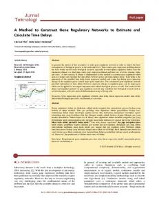
into account, but this would need more investigation and we consider it as part of our future work. Real Predicted

Throughput (KBytes/second)

Three different applications were used to validate the proposed approach. Each one included a different number of variables, variable classes and variable update rates. The real traffic for each application was then compared to the generated traffic models in terms of: number of packets, packet sizes, throughput, and packet inter-arrival time. For evaluating errors between the predicted and the real traffic we used the Mean Absolute Percentage Error (MAPE). According to Lewis (1982) [6], the lower the MAPE the more accurate the forecast. This way, it is considered that a MAPE value less than 10% shows a high accuracy, while between 11% and 20% we can assume a good result. A result between 21% and 50% is considered reasonable. However, in case the error is larger than 51% it can be a clear indicator of inaccuracy. Throughout the validation process we used the following equation to calculate MAPE: n 100 X Rt − Pt , (1) n t=1 Rt

4.0

Application 3

3.5

Application 2

3.0

Application 1

where Rt is the real value in period t, Pt is the predicted value in period t and n is the number of periods used in the calculations. 4.1 Number of packets As shown in Table 2 the calculated error for the predicted number of packets is smaller than 1%. This is because even if the number of variables, variable classes and variable update rates are different for each application, variables can be placed in the same request, and will generate the same number of packets. 4.2 Packets sizes For the second and third application, packet sizes are exactly the same in the predicted and real applications, giving an error of 0%. Due to the fact that the analyzed protocol has a dynamic field, i.e. the sequence number, which can change its size, for the first application we recorded an error of 48.16%. At this point the proposed algorithm does not take into account the variation of packet sizes, and this is why almost half of the real packets from the first application have a different size. However, an improved version of the algorithm can take dynamic sizes

2.5 0

40

80

120

160

Capture snapshot (seconds)

200

Figure 4. Comparison of throughput between predicted & real traffic

4.3 Throughput The predicted throughput can be extracted by splitting the output of the algorithm in blocks of one second and summing the number of bytes. The following equation shows how to obtain the throughput for a specific second: X T hroughput(secondx) = |Plength | : secondx ≤ Ptime < secondx+1 .

(2)

As shown in Table 2, in all cases the average through-

CDF 500ms update rate

0.8

0.8

0.8

0.6 0.4

0 0.045

0.6 0.4 0.2

0.05

0.5

0.505

Time(seconds)

CDF 3s update rate

0.6 0.4 0.2

0 0.495

0.055

Time(seconds)

0 0.995

1

1.005

Time(seconds)

CDF 6s update rate 1

0.8

0.8 Percentage

1

0.6 0.4 0.2 0 2.995

Percentage

1

0.2

Percentage

CDF 1s update rate

1

Percentage

Percentage

CDF 50ms update rate 1

Predicted one Application 1 Application 2 Application 3

0.6 0.4 0.2

3 Time(seconds)

3.005

0 5.995

6

6.005

Time(seconds)

Figure 5. The calculated Cumulative Distribution Function (CDF) for each update rate put error is smaller than 2%, demonstrating the accuracy of the proposed algorithm. However, the maximum throughput errors are bigger than 41%, while the minimum throughput error for the first application is about 2321%. These maximum values are due to real system operations in which transmission times can be delayed, leading to a drop in the throughput value. In the next seconds these are followed by transmissions of the missed packets, leading to an increase in the throughput value. Consequently, the measured errors in some cases increase to large values. However, in the next seconds the error drops back to values smaller than 2%. A clear example of this behavior is also shown in Figure 4, where in the case of application 1 we can see a drop in the throughput, followed by a peak. 4.4 Packet inter-arrival time All the errors we measured for packet inter-arrival time were smaller than 10% and in most cases the error was less than 1%. As expected, the largest error was measured for the smallest update rate, i.e. 50ms, that is mainly due to the non-real-time OS we used to run the SCADA server and due to network delays. In order to estimate the distribution of packets in the predicted and real traffic, we also

calculated the Cumulative Distribution Function (CDF), shown in Figure 5. These figures show the accuracy of the predicted and of real applications for the configured system update rates. In each figure the horizontal axis is a ten milliseconds time interval (given in seconds), while the vertical axis represents the percentage of packets for each system update rate. As we can clearly see in Figure 5, the largest difference between the predicted and real packet distributions is for a 50ms update rate. The reason for this was already discussed in the previous paragraph and it can also be justified by looking at the measured errors in Table 2. The following figures show a more accurate CDF with the increase of the system update rate. By inspecting these figures we also notice that packet distributions can be specific to each application. In fact, in order to predict more accurately the small variations in the distribution that we can see in each case, the proposed algorithm used a Gaussian distribution function. This way we increased the accuracy of the approach and, as already discussed, we managed to obtain an error of less than 1% in most of the cases. Nevertheless, we believe that the algorithm can be further improved in order to take into account more application-specific variations and to further reduce all er-

rors below 1%.

5 Conclusions and future work Recent approaches in the field of Process Control System (PCS) traffic modeling [7, 9, 3] proved that the construction of accurate network traffic models is a difficult task. The time and resources required to construct realistic models constitute one of the biggest issues that engineers must solve. On the other hand, the automated model construction based on SCADA application characteristics can effectively eliminate these issues. Therefore, this paper proposes an approach to generate network traffic models for PCSs, starting from application-specific data such as the number of variables, variable types and variable update rates. Our main contribution is an algorithm that takes as input an application description and generates a traffic model of a given duration. The algorithm was constructed by inspecting the network traffic taken from a real SCADA installation including several applications. As shown by experimental results, the algorithm is highly accurate and it can predict the number of packets by an error < 1%, the packet sizes by an error of 0%, the throughput by an error < 2% and the packet inter-arrival time by an error < 10%. The main advantage of the proposed approach is that traffic models can be re-generated easily if needed, without having to analyze real traffic or to develop new models. Furthermore, the approach can be applied in several directions, starting from Intrusion Detection Systems, to the recreation of network traffic in simulated/experimental environments. As future work, we intend to apply the approach in the previously mentioned fields and to enhance it with application-specific analysis in order to further reduce errors in all measured cases below 1%.

[6]

[7]

[8]

[9]

[10]

[11]

[12]

[13]

[14]

Acknowledgements I˜naki Garitano is supported by the grant BFI09.321 of the Department of Research, Education and Universities of the Basque Government.

References [1] Scapy. http://www.secdev.org/projects/ scapy/, 2012. [Online; accessed March 22, 2012]. [2] Tcpdump & libpcap. http://www.tcpdump.org, 2012. [Online; accessed March 22, 2012]. [3] S. Cheung, B. Dutertre, M. Fong, U. Lindqvist, K. Skinner, and A. Valdes. Using model-based intrusion detection for scada networks. Proceedings of the SCADA Security Scientific Symposium, 2006. [4] P. D¨ussel, C. Gehl, P. Laskov, J.-U. Bußer, C. Strmann, and J. Kstner. Cyber-critical infrastructure protection using real-time payload-based anomaly detection. Critical Information Infrastructures Security, 6027:85–97, 2010. [5] N. Falliere, L. O. Murchu, and E. Chien. W32.stuxnet dossier. http://www.symantec.com/content/

[15]

en/us/enterprise/media/security_ response/whitepapers/w32_stuxnet_ dossier.pdf, February, 2011. [Online; accessed February 28, 2012]. K. D. Lawrence, R. K. Klimberg, and S. M. Lawrence. Fundamentals of forecasting using excel. Industrial Pr, 2008. A. N. Mahmood, C. Leckie, J. Hu, Z. Tari, and M. Atiquzzaman. Network traffic analysis and scada security. Handbook of Information and Communication Security, pages 383–405, 2010. McAfee Foundstone Professional Services and McAfee Labs. Global energy cyberattacks: ”night dragon”. http://heartland.org/sites/all/ modules/custom/heartland_migration/ files/pdfs/29423.pdf, February 10, 2011. [Online; accessed March 23, 2012]. T. Roosta, D. K. Nilsson, U. Lindqvist, and A. Valdes. An intrusion detection system for wireless process control systems. In 5th IEEE International Conference on Mobile Ad Hoc and Sensor Systems, 2008. MASS 2008, pages 866–872. IEEE, 2008. C. Siaterlis, A. P. Garcia, and B. Genge. On the use of emulab testbeds for scientifically rigorous experiments. IEEE Communications Surveys and Tutorials, 2012. Accepted. Symantec. W32.duqu the precursor to the next stuxnet. http://www.symantec.com/content/en/ us/enterprise/media/security_response/ whitepapers/w32_duqu_the_precursor_to_ the_next_stuxnet.pdf, November 23, 2011. [Online; accessed February 28, 2012]. The MathWorks Inc. Matlab - the language of technical computing. http://www.mathworks.com/ products/matlab/, 2012. [Online; accessed March 04, 2012]. The University of Utah. Emulab bibliography. http:// www.emulab.net/expubs.php, February 28, 2012. [Online; accessed March 04, 2012]. A. Valdes and S. Cheung. Communication pattern anomaly detection in process control systems. In IEEE Conference on Technologies for Homeland Security, 2009. HST’09., pages 22–29. IEEE, 11-12/04/2009 2009. B. White, J. Lepreau, L. Stoller, R. Ricci, S. Guruprasad, M. Newbold, M. Hibler, C. Barb, and A. Joglekar. An integrated experimental environment for distributed systems and networks. ACM SIGOPS Operating Systems Review, 36(SI):255–270, 2002.