A Method to Ensure Preference Consistency in ... - Semantic Scholar

Michael Kulok Graduate Research Assistant

Kemper Lewis

1

Professor Mem. ASME e-mail: [email protected] Department of Mechanical and Aerospace Engineering, University at Buffalo-SUNY, Buffalo, NY 14260

1

A Method to Ensure Preference Consistency in Multi-Attribute Selection Decisions A number of approaches for multi-attribute selection decisions exist, each with certain advantages and disadvantages. One method that has recently been developed, called the hypothetical equivalents and inequivalents method (HEIM) supports a decision maker (DM) by implicitly determining the importances a DM places on attributes using a series of simple preference statements. In this and other multi-attribute selection methods, establishing consistent preferences is critical in order for a DM to be confident in his/her decision and its validity. In this paper, a general preference consistency method is developed, which is used to ensure that a consistent preference structure exists for a given DM. The method is demonstrated as part of HEIM, but is generalizable to any cardinal or ordinal preference structure, where the preferences can be over alternatives or attributes. These structures play an important role in making selection decisions in engineering design including selecting design concepts, materials, manufacturing processes, and configurations, among others. The theoretical foundations of the method are developed and the need for consistent preferences is illustrated in the application to a drill selection case study where the decision maker expresses inconsistent preferences. 关DOI: 10.1115/1.2761921兴

Introduction

There are typically tradeoffs in decision making. Product design requires making a series of tradeoff decisions, including the rigorous evaluation and comparison of design alternatives using multiple, conflicting design criteria, or attributes. We can be certain that no one alternative will be best in every attribute. Therefore, how to make the “best” decision when choosing from among a set of alternatives in a design process has been a common problem in research and application in product design and development. While in conceptual design, the objective may be to identify a set of promising concepts, the discussion and context of this work focus on the decisions in design where a single concept must be selected. A number of methods have been developed to support this type of decision by capturing and quantifying decision maker preferences, such as the analytical hierarchy process 关1兴, utility theory 关2–4兴, discrete-choice analysis 关5兴, and conjoint analysis 关6兴. In general, the multi-attribute decision problem can be formulated as follows: Choose an alternative j so as to

冋兺 册 n

Maximize V共j兲 =

i=1

n

Subject to

1/s

共wiaijs兲

共1兲

兺w =1 i

i=1

where V共j兲 is the value function for alternative j, wi is the weight for attribute i, and aij is the normalized rating of alternative j on attribute i. The parameter s can be interpreted as a measure of compensation, or tradeoff. Higher values of s indicate a greater 1 Corresponding author. Contributed by the Design Automation Committee of ASME for publication in the JOURNAL OF MECHANICAL DESIGN. Manuscript received July 20, 2006; final manuscript received December 18, 2006. Review conducted by Timothy W. Simpson. Paper presented at the ASME 2005 Design Engineering Technical Conferences and Computers and Information in Engineering Conference 共DETC2005兲, Long Beach, CA, September 24–28, 2005.

1002 / Vol. 129, OCTOBER 2007

willingness to allow high preference for one criterion to compensate for lower values of another 共see an extensive discussion of the implications of the parameter s in 关7兴兲. The value function in Eq. 共1兲 is a simplified version of a general aggregation function 关7,8兴, assuming that the sum of weights is always equal to one. The general aggregation function that provides the basis for Eq. 共1兲 satisfies a set of axioms that an aggregation function, appropriate for rational design decision making, must obey 关9兴. Note that when s = 1, Eq. 共1兲 becomes a L1-norm and when s = 2, Eq. 共1兲 becomes a L2-norm. For a vector of ratings, ¯x = 共x1 ¯ xn兲T, and a ¯ = 共w1 ¯ wn兲T, the L1-norm is the weighted vector of weights, w n n wix2i sum 兺i=1wixi, and the L2-norm is the Euclidean-norm 冑兺i=1 关10兴. By using a general weighted mean aggregation function, it is necessary to assume that the attributes are mutually and preferentially independent 关2兴. While this is not always true of engineering design problems, there are conditions that effectively weaken these necessary assumptions when the number of attributes is four or more, as noted on p. 112 of 关2兴. In addition, as noted in Claim 4.2 of 关8兴, the limit of the weighted mean aggregation function as s approaches zero is the weighted product of the powers aggregation function, which would then not require the mutually and preferentially independent assumption. While a study of the s parameter is beyond the scope of this paper, it is important to note the limitations and possibilities of using a general aggregation function of Eq. 共1兲. There are many ways to implement and solve this formulation. Most methods focus on formulating the attribute weights wi and/or the alternative scores aij, indirectly or directly from the decision maker’s preferences. In new product development, a common challenge in a design process is how to capture the preferences of the end-users while also reflecting the interests of the designer共s兲 and producer共s兲. Typically, preferences of end-users are multidimensional and multi-attribute in nature. If companies fail to satisfy the preferences of the end-user, the product’s potential in the marketplace will be severely limited. In this paper, we focus on the soundness and consistency of the process of making these decisions. Indeed, when seven alternatives are ranked using multiple attributes, the process used to make the decision influ-

Copyright © 2007 by ASME

Transactions of the ASME

Downloaded 25 Mar 2008 to 128.205.213.117. Redistribution subject to ASME license or copyright; see http://www.asme.org/terms/Terms_Use.cfm

ences the outcome over 93% of the time 关11兴. Since the process by which the decision is made plays such an important role, establishing a theoretically sound decision process is paramount in identifying the correct outcome. As noted in 关2兴, in the context of multi-attribute utility function formulation, checking for and establishing consistency in decision maker preferences is vital to ensure reliable and effective decisions. In this paper, we develop a novel approach to check and ensure the preference consistency of a single decision maker. While the approach can be used in a number of contexts within general multi-attribute selection decisions, including the 共ordinal or cardinal兲 comparison of alternatives or attributes, we demonstrate its development and application using ordinal alternative comparison. There are a number of approaches to make multi-attribute selection decisions; many of the possible methods and their theoretical or empirical limitations are discussed in 关12兴. Only a subset of the methods and limitations that are relevant to this work are presented in this paper. The pairwise comparison method takes two alternatives at a time and compares them to each other in a tournament type of approach until one winning alternative is identified. A pairwise approach is used in the analytic hierarchy process 共AHP兲 to find relative importances among attributes 关1兴. Adaptations of AHP and other pair-wise methods are widely used to obtain relative attribute importances 关13兴, to select from competing alternatives 关14,15兴, and to aggregate individual preferences 关16,17兴. There are two fundamental limitations in using pairwise comparisons to make these decisions. First, they ignore the true value functions 共also known as utility functions, preference functions, or worth functions兲 of a decision maker, which are many times nonlinear. Second, when comparing, they do not directly account for the relative importance of the attributes. Because of these limitations, there exists some level of uncertainty when evaluating pairs of alternatives. This uncertainty is studied in the context of preference consistency in 关18兴. While some details exist regarding the theoretical problems with pairwise comparisons 关10,19,20兴, under certain assumptions, some adaptations of pairwise comparisons can provide effective and practically useful results 关21兴. Rankings are commonly used to rank order a set of alternatives. U.S. News and World Report annually ranks colleges based upon a number of attributes 关22兴. The NCAA athletic polls are based on a ranking system. Compared with standard pairwise methods, ranking methods are slightly more elaborate. However, as shown in 关23,24兴, the ranking procedure violates the independence of irrelevant alternatives principle, which states that the option chosen should not be influenced by irrelevant alternatives or clear noncontenders. Ranking approaches are prone to rank reversals when alternatives are dropped from consideration. However, it is noted in 关25兴 that the probability and impact of rank reversals when using ranking systems is quite low. Also, when rankings are used, it is difficult to ascertain the importance of the various attributes that were used to obtain the rankings. In general, determining the relative importance of the attributes in a selection problem is largely an arbitrary process. This arbitrary process can create a number of complications in multiattribute decision making and optimization 关26–29兴. In previous work, we have developed an approach called the hypothetical equivalents and inequivalents method 共HEIM兲 to analytically determine these weights using a decision maker’s stated preferences over a set of hypothetical alternatives 关24兴. HEIM expands the concepts of indifference relationships found in 关30,31兴, and has since been effectively expanded to identify a single, robust solution 关32兴, handle alternatives with uncertain attributes 关33兴, and to support group decision making 关34兴. HEIM is similar to multi-attribute approaches described in 关2,31兴 in that it uses stated equality preferences from the decision maker based on hypothetical alternatives. However, HEIM is unique because it accommodates inequality preference statements and is easily scalable to problems with many attributes because it Journal of Mechanical Design

avoids having to address preferential independence or reduction of dimensionality when there are three or more attributes. While the details of HEIM are given in 关24兴, a brief summary is given here to put the remainder of the paper in proper context. The basic premise of HEIM is to elicit preferences from a decision maker on pairs of hypothetical alternatives. Hypothetical alternatives have the same set of attributes as the actual alternatives, but differ in the combinations of attribute values. This is done to determine the attribute weights while avoiding any bias the decision maker may have towards the actual alternatives. The “equivalents” part of the method allows a decision maker to make statements like “hypothetical alternatives A and B are equivalent in value to me.” By making this kind of statement, a decision maker is identifying an indifference relationship between A and B. However, finding hypothetical equivalents that are exactly of equivalent value to a decision maker, or “indifference points,” can be a challenging and time-consuming task 关35兴, specifically in the context of constructing utility functions. Therefore, HEIM also accommodates inequivalents in the form of stated preferences such as “I prefer hypothetical alternative A over B.” When a preference is stated, by either equivalence or inequivalence, a constraint is formulated and an optimization problem is constructed to solve for the attribute weights. The weights are solved by formulating the following optimization problem:

冉

Minimize

f共x兲 = 1 −

n

兺

wi

i=1

冊

2

Subject to h共x兲 = 0

共2兲

g共x兲 ⱕ 0 where the objective function ensures that the sum of the weights is equal to one. X is the vector of attribute weights, n is the number of attributes, and wi is the weight of attribute i. The constraints are based on a set of stated preferences from the decision maker. The equality constraints are developed based on the stated preference of “I prefer alternatives A and B equally.” In other words, the value of these alternatives is equal, giving the following equality constraint: h:V共A兲 = V共B兲

or h:V共A兲 − V共B兲 = 0

共3兲

The inequality constraints are developed based on the stated preference of “I prefer A over B.” In other words, the value of alternative A is more than alternative B, as shown in the inequality constraint in Eq. 共4兲: g:V共A兲 ⬎ V共B兲

or g:V共B兲 − V共A兲 ⬍ 0

共4兲

An important facet of the HEIM approach and other decision making approaches is the assumption of consistent preferences on the behalf of the decision maker. For instance, if a decision maker states that they prefer A over B, B over C, and C over A, they are not consistent, since the preferences structure would be A Ɑ B Ɑ C Ɑ A where “Ɑ” means “preferred to.” This structure would lead to the following set of constraints: V共A兲 ⬎ V共B兲 V共B兲 ⬎ V共A兲 V共A兲 ⬎ V共C兲 V共C兲 ⬎ V共A兲 V共B兲 ⬎ V共C兲 Since the first two sets of constraints are inconsistent, this structure leaves most decision making approaches and the decision maker in a situation where no solution can be found and no decision can be made. It may appear that developing a set of inconsistent preferences would be rather difficult for a rational decision maker and the case described above may be rare. However, in 关36兴, 80 decision makers were asked the same 100 pairwise comparison questions on two separate occasions with 3–5 days of separation, and the consistency rates for each person ranged from 60–90%. As concluded in 关36兴, the respondents were certainly not OCTOBER 2007, Vol. 129 / 1003

Downloaded 25 Mar 2008 to 128.205.213.117. Redistribution subject to ASME license or copyright; see http://www.asme.org/terms/Terms_Use.cfm

answering the questions randomly, else the consistency rate would have been around 50% 共since there is a 50% chance that the random answers to any of the 100 questions from both rounds would match兲. In another study 关37兴, subjects were asked the same 42 questions twice, with the second time coming immediately after the first time. Consistency rates were well under 100%. The economic choice theory researchers concluded in 关38兴 that the most likely source of these inconsistencies was “stochastic choice,” or what one might call “error” or “mistakes” on the part of the decision makers. In addition, as noted in 关39兴, people struggle with the internal consistency of decisions and the empirical accuracy of decisions based on multiple fallible indicators. It is argued in 关39兴 that the integration of consistency and accuracy be viewed in the context of rationality. Identifying these inconsistencies or “mistakes” as denoted in 关38兴, and correcting them is one of the primary objectives of the work in this paper. Developing consistency checks for preferences is one way to promote rational and reliable decisions. In the method described in 关40兴, a least-distance approximation method using pairwise preference information attempts to account for inconsistent preferences by introducing “slack” variables to represent the inconsistency. The inconsistency is minimized; however, it may not be eliminated. We take a different approach in this paper and develop a method that identifies and eliminates the inconsistency before a decision is made. Other consistency methods have been developed for assessing attribute importances 关1兴, multi-attribute utility functions 关2兴, preferences for rational altruistic behavior 关41兴, and the transformation between multiplicative and fuzzy preference models 关42兴. The consistency check in 关1兴 uses an arbitrary scale to make paired comparisons among alternatives 共e.g., 兵9 , 8 , 7 , 6 , 5 , 4 , 3 , 2 , 1 , 21 , 31 , 41 , 51 , 61 , 71 , 81 , 91 其兲 and then makes use of a subjective criterion to determine if a set of alternative preferences is consistent or not 共e.g., the consistency ratio must be less than 10%兲. The consistency method presented in this work uses meaningful scales to make marginal rates of substitution comparisons among attributes, and then uses an objective criterion to determine if a set of alternative preferences is consistent or not, using both the alternative and attribute comparisons. Our mindset is that a decision maker is either consistent or not, while the approach in 关1兴 allows a range of inconsistency to be deemed “consistent” due to the arbitrary nature of the comparison scales. In the next section, the fundamentals of the preference consistency check are presented. Then, the approach is applied to a multi-attribute selection problem where an actual professional construction contractor is used as the decision maker to exercise the consistency check procedure. Finally, we close the paper with a set of observations and conclusions.

2

The Preference Consistency Method

As demonstrated in the previous section, a number of multiattribute decision methods are based on evaluating the relative value of alternatives or attributes. Pairwise comparisons compare two alternatives at a time. AHP uses pairwise comparisons to compare attributes. Ranking methods provide cardinal comparisons of alternatives. HEIM elicits preferences from a decision maker on hypothetical alternatives. In each of these methods, consistency is critical to being able to identify a preferred alternative with confidence. In this section, a preference consistency method is developed that can be applied to any ordinal or cardinal set of preferences. In Sec. 3, the method will be demonstrated as part of HEIM to illustrate its usefulness. 2.1 Fundamental Model. For simplicity and without any loss of generality, we will use a simple two-alternative preference to illustrate the development of the preference consistency method. In addition, the value of a given alternative can take a number of forms, including the general form shown in Eq. 共1兲. In this work, 1004 / Vol. 129, OCTOBER 2007

we use the additive form 共L1-norm兲 because it demonstrates the preference consistency approach well and because of its prominence in engineering design applications. Assume that the DM prefers alternative B over C. Using Eq. 共4兲, this assumed preference, although the values of each alternative are unknown at this point, can be expressed as shown in Eq. 共5a兲. Using the L1-norm representation of value, Eq. 共5a兲 can then be refined as shown in Eq. 共5b兲: V共C兲 ⬍ V共B兲 n

兺wa

i iC

i=1

共5a兲

n

⬍

兺wa

共5b兲

i iB

i=1

Since the value of alternative B is larger 共only in an ordinal sense兲 than the value of alternative C, in order to make the alternatives of equal value, some 共unknown兲 quantity of value must be added to C. The quantity may change depending upon the form of the value aggregation function used, but some quantity, greater than zero, must be added. While the L1-norm form of the weighted mean aggregation function is illustrated in Eq. 共5b兲 and in the following method development, the fundamental concepts apply regardless of the form of the aggregation function. We have made reference to the implications of using other forms of the aggregation function throughout the developments of Sec. 2. This addition of a unitless added value converts Eq. 共5兲 into an equality where the difference in value between alternatives C and B is expressed through the term ⌬V j,␣ where j specifies the lower valued alternative that an amount of value ⌬V is being added to, and ␣ specifies the higher valued alternative, as shown in Eq. 共6兲: n

兺 i=1

n

wiaiC + ⌬VC,B =

兺wa

i iB

共6兲

i=1

The exact quantity ⌬V j,␣ is not of paramount concern here; indeed, Eq. 共5兲 is a form of an ordinal scale and therefore, we are not concerned with transforming it into a cardinal scale. However, the sign of the quantity is important to maintain the ordinal structure, and is the focus of the remainder of the approach. According to the preference structure of the DM, ⌬VC,B as defined must be positive, which is critical in the development of the consistency check. Since there are n attributes in this selection problem, the increase of value of alternative C can come from an increase in any of the attributes or some combination of the attributes. We assume the additional value is expressed by an increase in only one attribute, while the other attributes are kept at their current levels to simplify the derivation and approach. Note that we assume that the attributes are positively oriented such that the value of an alternative increases as an attribute increases. There may be some cases where the increase in only one attribute may not increase the value of one alternative enough. In these cases, an increase in a second attribute can also be used. The method would then be applied twice, once to the increase in the first attribute and again to the increase in the second attribute. However, we present the derivation assuming only one attribute is being used. The additional value added to alternative j to make it equal to alternative ␣ 共⌬V j,␣兲 can be expressed by an increase in attribute i multiplied by the attribute weight wi as shown in Eq. 共7兲. This increase in the attribute i is denoted as ki,j,␣, the consistency indicator: ⌬V j,␣ = ki,j,␣wi

共7兲

When using the L1-norm 共s = 1兲, ki,j,␣ is simply the increase in a given attribute i to bring alternative j equal in value to alternative ␣. More generally, when using any form of the weighted mean in Eq. 共1兲, ki,j,␣ is found using the binomial theorem and is given in Eq. 共8兲: Transactions of the ASME

Downloaded 25 Mar 2008 to 128.205.213.117. Redistribution subject to ASME license or copyright; see http://www.asme.org/terms/Terms_Use.cfm

s

ki,j,␣ =

兺 t=0

冋冉 冊 册 s t

ait⌬ais−t − ais

For the L1-norm example in Eq. 共6兲, this additional value ⌬VC,B is then expressed by an increase in attribute i 共ki,C,B兲 multiplied by the attribute weight wi, and shown in Eq. 共9兲: n

兺

n

wiaiC + ki,C,Bwi =

i=1

兺wa

i iB

⳵V ⌬alj ⳵ aij wi ␭ilj = − = = ⌬aij ⳵ V wl ⳵ alj

冏冏

共8兲

共9兲

These MRSs can be used in Eq. 共10兲 to reduce the number of unknowns to one 共k1,C,B兲 by substituting the following terms on the left side of Eq. 共10兲 共alternative C兲:

i=1

Since ⌬VC,B ⬎ 0, and by definition all attribute weights are nonnegative, ki,C,B must also be positive. If ki,C,B were negative, this would indicate that ⌬VC,B ⬎ 0, and subsequently, V共C兲 ⬎ V共B兲, which violates the DM stated preference of alternative B over C. Therefore, determining the sign of the ki,j,␣ consistency indicator terms is the focus of the remaining part of the derivation. 2.2 Selection of ki,j,␣. To determine ki,j,␣, one attribute must be selected. Since ki,j,␣ indicates an increase in an attribute for a given alternative, the selected attribute should not already have a high satisfaction. As a general guideline, the attribute with the lowest satisfaction in the lower valued alternative can be chosen as the one to determine ki,j,␣. If there are two attributes with the same satisfaction, then either one can be chosen. In the general problem of Eq. 共9兲, assume that attribute 1 has the lowest value and is chosen as the attribute to add value to for alternative C. Eq. 共9兲 can now be written as: n

兺wa

i iC

n

+ k1,C,Bw1 =

i=1

兺wa

i iB

共10兲

2.3 Determining the Sign of ki,j,␣. While the numerical value of ki,j,␣ can be found, whether the value is positive or negative is most important. If ki,j,␣ is positive, then the preference statement is consistent; if ki,j,␣ is negative, then the preference statement is inconsistent. These conditions hold regardless of which form of the weighted mean aggregation function of Eq. 共1兲 is used. For different forms of the aggregation function, the numerical value of ki,j,␣ will change 共see Eq. 共8兲兲. However, the sign will not. When one alternative is preferred over another, that indicates that the preferred alternative has greater value than the other alternative regardless of what kind of aggregation function is used. The consistency indicator ki,j,␣ is determined using the concept of marginal rate of substitution 共MRS兲 关43兴, which captures how much of one attribute the DM is willing to sacrifice to gain a specific amount of another attribute. The MRS, or ␭ilj, can be expressed in Eq. 共11兲, where the term ⌬aij represents the amount of attribute l the DM is willing to sacrifice in order to gain an amount of ⌬aij on the attribute i for alternative j 共the negative sign is necessary because one of the ⌬a terms is always negative since it represents a sacrifice in one attribute for a gain in another兲. Since a DM usually has nonlinear value functions and MRS construction is typically done using the natural attribute units, we convert the MRS of attributes l and i for alternative j into normalized attribute ratings using Eq. 共11兲 关2兴. From the value function in Eq. 共1兲, the ratio of partial derivatives can also be expressed as a ratio of only wi and wl. As noted in 关2兴, Eq. 共11兲 implies 共and assumes兲 that the MRS relationship between any two relationships is linear—that the amount of one attribute that a decision maker is willing to sacrifice in order to gain a specified amount of another attribute is constant, regardless of the alternative in question 共alternative j in Eq. 共11兲兲. However, in engineering design, this is not typically the case. It is more common for the MRS evaluations between two attributes to depend upon the alternative in question. In this case, the MRS relationships can be linearized through a change of scale 共关2兴, pp. 86–90兲 Journal of Mechanical Design

w2 =

w1 w1 , . . . ,wn = ␭12C ␭1nC

共12兲

and the following terms on the right side of Eq. 共10兲 共alternative B兲: w2 =

w1 w1 , . . . ,wn = ␭12B ␭1nB

共13兲

resulting in Eq. 共14兲: a1Cw1 + a2C

w1 w1 + ¯ + anC + k1,C,Bw1 ␭12C ␭1nC

= a1Bw1 + a2B

w1 w1 + ¯ + anB ␭12B ␭1nB

共14兲

Now wl can be canceled, reducing Eq. 共14兲 to Eq. 共15兲 where the only unknown is kl,C,B: k1,C,B = a1B + a2B

i=1

Since the wi terms are still unknown, ki,C,B cannot be directly solved for yet.

共11兲 j

− anC

1 1 1 + ¯ + anB − a1C − a2C − ¯ ␭12B ␭1nB ␭12C

1 ␭1nC

共15兲

The total number of MRS evaluations necessary for Eq. 共15兲 is 关2共n − 1兲兴, where n is the number of attributes. For the more general case with ␤ unique preference statements in the form of Eq. 共5a兲, the total number of MRS evaluations necessary is bounded by 关2␤共n − 1兲兴. After solving for kl,C,B, there are three possible cases to consider: • • •

If k1,C,B ⬎ 0, the DM is consistent since this indicates that the indicated lower valued alternatives is indeed lower valued. If k1,C,B ⬍ 0, it indicates the DM is not consistent and this preference statement is not correct since the indicated lower valued alternative is actually the higher valued alternative. If k1,C,B = 0, it indicates that the DM is not consistent and that the alternatives are actually of equal value. In this case, the preference state should be one of equality 共an equality constraint兲.

When the preference statement is changed in the last two cases, it should be evaluated by the DM and then the consistency method must be run again. This ensures that the new preference has not created any other inconsistencies. When the preference statements are changed, it is important to include the DM in the process of “introspection,” so that he can reconsider his needs, new information, and the ramifications of the proposed changes 关44兴. These conclusions are also based on the assumption that the value functions are correct and that the MRS evaluations are correct. There are some general guidelines to ensure that the MRS evaluations were performed correctly including: 共1兲 ␭ilj = 1 / ␭lij: If done correctly and consistently, the amount the DM is willing to sacrifice on attribute i for a gain in attribute l, should be the reciprocal of the amount the DM is willing to sacrifice on attribute l for a gain in attribute i. This is similar to the reciprocal scale used in 关1兴 to compare alternatives, but by using MRS evaluations, meaningful OCTOBER 2007, Vol. 129 / 1005

Downloaded 25 Mar 2008 to 128.205.213.117. Redistribution subject to ASME license or copyright; see http://www.asme.org/terms/Terms_Use.cfm

Table 1 The 18 drill alternatives Drill No. 1 2 3 4 5 6 7 8 9 10 11 12 13 14 15 16 17 18

Number of operations

Price 共$兲

Weight 共lb兲

350 370 380 400 420 430 450 470 480 500 520 530 550 570 580 600 620 630

70 80 85 72 82 88 74 85 91 79 89 94 84 93 97 90 98 100

6.0 5.7 5.5 6.5 6.1 5.8 6.9 6.5 6.1 7.2 6.9 9.4 7.5 7.2 6.7 7.8 7.5 7.0

scaled comparisons are used for the attributes in order to assess preference consistency for the alternatives. 共2兲 If the DM can rank order the attributes and if attribute i is more important than attribute l, then ␭ilm = wi / wl ⬎ 1. For all pairs of attributes where one is more important than another, this relationship should hold. 共3兲 More formal evaluation and convergence routines can be used, as described in 关45兴. In the next section, the complete HEIM approach, including the preference consistency method, is demonstrated on a drill selection problem. A lead construction engineer from a local construction firm is used as the DM and to provide insight into the final selected drill and its implications.

3

Drill Selection Problem

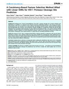
3.1 Problem Setup. Although the method is discussed in this section in the context of the HEIM approach, it can be applied to any ordinal or cardinal set of preferences. To illustrate the application of the method, assume a decision maker has to select a drill from the following set of cordless drills shown in Table 1 关46兴. The attributes of interest are the number of operations, the price, and the weight. A construction engineer is used as the decision maker. Using a midvalue splitting technique 关2兴, value functions for each attribute across each attribute range were developed with the DM and are shown in Fig. 1. As part of the HEIM approach, a set of hypothetical alternatives 共hypothetical drills兲 are developed and are shown in Table 2. These hypothetical alternatives are developed in such a way to sample the complete attribute space in an ordered, balanced way using an L9 orthogonal array 关47兴. The attribute space is defined by the maximum and minimum attribute values of the actual alternatives in Table 1 共350–630 for number of operations, $70–$100 for price, and 5.5 lb–9.4 lb for weight兲. The L9 array results in nine alternatives with the normalized attribute combinations, where 0 indicates the lowest value for the attribute and 1 indicates the highest value for the attribute, shown in Table 2. The last column represents the value of the alternative using the additive value function, as given in Eq. 共1兲. The hypothetical alternatives of Table 2 are converted into natural unit alternatives, using the value functions in Fig. 1. For instance, for hypothetical alternative D, the number of operations is 0, indicating the lowest value for the number of operations, or 350. The price is set at 0.5, and from the middle graph of Fig. 1, this corresponds to a price of $90. The weight is set at 0.5 and from the bottom graph of Fig. 1, this corresponds to a weight of 7.0 lb. The other hypothetical alternatives are developed in a simi1006 / Vol. 129, OCTOBER 2007

Fig. 1 Value function representations

lar fashion and are partitioned into three sets of three alternatives in Table 3. This makes it easier for the DM to express preferences over a set of three alternatives instead of all nine alternatives. An important issue to consider when partitioning the alternatives is to make sure that useful comparisons can be made between alternatives. For instance, it would not be useful to develop a subset where one alternative is clearly better than the other alternatives across all of the alternatives. Different possible partitions are certainly possible, but as long as decision maker consistency is maintained, different partitions should lead to the same solution. The partitioning issue is expanded upon in 关32兴 and continues to be an area of current study. 3.2

Developing Preference Structures. In the next step, the Transactions of the ASME

Downloaded 25 Mar 2008 to 128.205.213.117. Redistribution subject to ASME license or copyright; see http://www.asme.org/terms/Terms_Use.cfm

Table 2 Hypothetical alternatives Hypothetical alternative A B C D E F G H I

Number of operations

Price

Weight

0 0.5 1 0 0.5 1 0 0.5 1

0 0.5 1 0.5 1 0 1 0 0.5

0 1 0.5 0.5 0 1 1 0.5 0

Table 5 Different representations of the preferences

Value of alternative

Preference statements

0 0.5w1 + 0.5w2 + w3 w1 + w2 + 0.5w3 0.5w2 + 0.5w3 0.5w1 + w2 w1 + w3 w2 + w3 0.5w1 + 0.5w3 w1 + 0.5w2

CⱮB

preference statements of the DM for each set have to be determined, which are given in Table 4. The preference statements B Ɑ A and C Ɑ A do not add any valuable information, since alternative A is dominated by every other alternative. Therefore, the statements with alternative A are not included in the analysis. From Table 4, five unique preference statements can be derived, which are listed in Table 5, including their representation in terms of values and the resulting inequality constraints. All the other constraints from Table 4 are redundant to those listed in Table 5. Investigating the inequality constraints, it is apparent that the C Ɱ B constraint is the direct opposite of the D Ɱ E constraint. This means that the DM is inconsistent and that either the C Ɱ B preference statement or the D Ɱ E preference statement must be incorrect. Without further analysis, it is difficult to determine which statement is wrong. To find out which of them is incorrect, the preference consistency method can be applied. Note that if these constraints were used in an optimization formulation 共e.g., Eq. 共2兲兲, there would be no feasible 共or optimal兲 solution. 3.3 Application of the Preference Consistency Method. From the value equations in Table 5 共second column兲 the ki,j,␣ terms shown in Table 6 are chosen to represent the value increases based on the worse attribute of the lower-valued alternative. For example, for the preference, C Ɱ B, the first and second attributes for alternative C are already at their highest satisfaction level 共coTable 3 Sets of hypothetical alternatives Alternatives

Number of operations

Price

Weight

100 90 70

7.8 5.5 7

90 70 100

7 7.8 5.5

Set 1 A B C

350 500 630

Preference statements in value levels w1 + w2 + 0.5w3⬍ 0.5w1 + 0.5w2 + w3 0.5w2 + 0.5w3⬍ 0.5w1 + w2 0.5w1 + w2 ⬍ w1 + w3 w2 + w3 ⬍ w1 + 0.5w2 w1 + 0.5w2⬍ 0.5w1 + 0.5w3

DⱮE EⱮF GⱮI IⱮH

Inequality constraints 0.5w1 + 0.5w2 − 0.5w3 ⬍ 0 −0.5w1 − 0.5w2 + 0.5w3 ⬍ 0 −0.5w1 + w2 − w3 ⬍ 0 −w1 + 0.5w2 + w3 ⬍ 0 0.5w1 + 0.5w2 − 0.5w3 ⬍ 0

efficient of 1 for w1 and w2兲, and so attribute three is chosen 共k3,C,B兲. At this point, the lower bound of each ⌬V j,␣, ⌬Vmin j,␣ , is , is unknown. zero and the upper bound of each ⌬V j,␣, ⌬Vmax j,␣ In the next step, the MRS’s have to be determined to calculate the consistency indicators in Table 6. The DM was asked for a series of MRS values, similar to the example form shown in Table 7. In this form, the DM is asked to determine for alternative B how many operations he is willing to sacrifice for a 1 lb decrease in weight, and how much more he is willing to pay for the same 1 lb decrease in weight. Note that this is a cross-attribute preference assessment, as opposed to the value functions shown in Fig. 1, which only capture preferences on each attribute individually. This cross-attribute tradeoff assessment is critical to determine the consistency of the statements in Table 4, since the DM implicitly processes attribute tradeoffs when stating their preferences over the hypothetical alternatives. Using the value functions of Fig. 1 and Eq. 共10兲, the MRS responses are converted to unitless MRS values, as shown in Table 8. Using these MRS values in a similar manner to the approach outlined in Sec. 2.3, the consistency indicators are solved for and shown in Table 9. From the data in Table 9, it can be concluded that the preference statements C Ɱ B and I Ɱ H are incorrect, since they are negative. This is not surprising, since the constraints for these preferences in Table 9 are exactly the same. If one were wrong, the other certainly must also be wrong. This means that these two preference statements have to be switched to C Ɑ B and I ⬎ H. With these new preferences, two new consistency indicators are calculated using the MRSs from Table 8 共k1,B,C = 0.47, k1,H,I = 0.42兲, which indicates that the preference statements C Ɑ B and I Ɑ H are correct. Since the original preference statement H Ɑ I Ɑ G from Table 4 has been corrected to I Ɑ H Ɑ G, it also has to be examined if the preference statement H Ɑ G is correct. Using the same procedure, it was determined that this statement was incor-

Set 2 D E F

350 500 630 Set 3

G H I

350 500 630

70 100 90

5.5 7 7.8

Table 6

The consistency indicators ki,j,␣ for each preference

Preference statements

ki,j,␣

C⬍B D⬍E E⬍F G⬍I I⬍H

k3,C,B k1,D,E k3,E,F k1,G,I k3,I,H

Table 4 Preference statements for each set Set 1 2 3

Journal of Mechanical Design

Table 7 Example MRS form

Preference statements BⱭCⱭA FⱭEⱭD HⱭIⱭG

Alternative B ␭31B ␭32B

Number of operations 쏋

Price

Weight

쏋

−1 lb −1 lb

OCTOBER 2007, Vol. 129 / 1007

Downloaded 25 Mar 2008 to 128.205.213.117. Redistribution subject to ASME license or copyright; see http://www.asme.org/terms/Terms_Use.cfm

Table 8 MRS values for each alternative Alternative

MRS ␭31B = 0.67␭32B = 1.44 ␭31C = 0.71␭32C = 1.36 ␭12D = 2.09␭13D = 1.50 ␭12E = 1.97␭31E = 0.68 ␭12F = 2.05␭23F = 0.71 ␭12G = 1.95␭13G = 1.54 ␭31H = 0.65 ␭12I = 1.99␭31I = 0.64

B C D E F G H I

rect as well, and was switched to H Ɱ G. At this point, all the consistency indicators are positive, as shown in Table 10, indicating a set of consistent preferences. While it may seem that like these preference changes are being made without input or confirmation from the DM, this is not the case. The new preferences were developed using the input from the DM and were confirmed by the DM when we showed him the incorrect preferences. In fact, he stated that he was not quite sure why he initially stated his preferences that way, but agreed with the changes and corrections. This provides anecdotal evidence to the research studies on the mistakes that rational decision makers can make as discussed in 关36–38兴. The final preference statements and corresponding inequality constraints are given in Table 11. 3.4 Identifying the Best Alternative. Using the inequality constraints from Table 11, the optimization formulation in Eq. 共16兲 can be constructed in order to determine the attribute weights and the most preferred drill for the DM. There are only four inequality constraints, as the ones resulting from the preference statements B Ɱ C and E Ɱ D are redundant:

Table 9 Initial values of ki,j,␣ terms Preference statements

ki,j,␣

CⱮB DⱮE EⱮF GⱮI IⱮH

k3,C,B = −0.56 k1,D,E = 0.43 k3,E,F = 0.97 k1,G,I = 0.09 k3,I,H = −0.71 Table 10 Final values of the ki,j,␣ terms

Preference statements

ki,j,␣

CⱮB DⱮE EⱮF GⱮI IⱮH

k3C = 0.47 k1D = 0.43 k3E = 0.97 k1G = 0.09 k3I = 0.63

Table 11 Final preference structure and inequality constraints Preference statements BⱮC DⱮE EⱮF GⱮI HⱮG

Inequality constraints −0.5w1 − 0.5w2 + 0.5w3 ⬍ 0 −0.5w1 − 0.5w2 + 0.5w3 ⬍ 0 −0.5w1 + w2 − w3 ⬍ 0 −w1 + 0.5w2 + w3 ⬍ 0 0.5w1 − w2 − 0.5w3 ⬍ 0

1008 / Vol. 129, OCTOBER 2007

Fig. 2 Feasible design space

Minimize 共1 − 共w1 + w2 + w3兲兲2 Subject to g1: − 0.5w1 − 0.5w2 + 0.5w3 ⬍ 0 g2: − 0.5w1 + w2 − w3 ⬍ 0 g3: − w1 + 0.5w2 + w3 ⬍ 0

共16兲

g4: 0.5w1 − w2 − 0.5w3 ⬍ 0 0 ⱕ w1,w2,w3 ⱕ 1 In Eq. 共16兲, we are trying to find a set of weights that sum to one and that satisfy the constraints. However, there could exist multiple sets of weights that satisfy these criteria and are both feasible and optimal. In addition, these multiple sets of weights could result in a different drill being selected as the most preferred drill, as shown for other problems in another study 关32兴. This is not an advantageous consequence, as it leaves the DM without having identified a single, preferred choice. Therefore, the basic concepts of the method, that a quantifiable difference between two alternatives exists 共Eq. 共6兲兲, and that this difference can be formulated as an increase in a single attribute 共Eq. 共7兲兲, are used to identify the single most preferred drill, as described in the following discussion. In order to determine all the possible sets of feasible and optimal weights and their corresponding winnings drills, many combinations of weights are generated in the feasible space, as defined by the preference constraints and the constraint that the sum of the weights must equal one. A fine grid technique is used to generate the points. For each combination of weights, the value functions of all 18 drills are calculated and the winning drill is determined. As a result, unless all feasible and optimal combination of weights result in the same winning drill, there will be more than one winning drill. In Fig. 2, the feasible and optimal design space is shown where the large blue triangle represents the w1 + w2 + w3 = 1 plane and all the points lie on this plane 共the axes are shifted slightly to aid in visualizing the plot兲. The smaller triangular region of colored points represents the feasible design space, where only three of the four inequality constraints are active 共g2, g3, and g4兲. The five colored regions in the feasible space correspond to five different drills that have the highest values using the combinations of weights in that region. At this point, the DM has reduced the number of possible alternatives from 18 to five, but a single best drill has not been determined. However, from the boundaries of the feasible region, the maximum and minimum values of each weight can be found using the set of generated weight combinations. These ranges are shown in Table 12. While these ranges are visually apparent from the feasible space in Fig. 2, for problems with more than three attributes, these ranges are simply found from the set of feasible Transactions of the ASME

Downloaded 25 Mar 2008 to 128.205.213.117. Redistribution subject to ASME license or copyright; see http://www.asme.org/terms/Terms_Use.cfm

Table 12 Minimum and maximum weights

w1 w2 w3

Minimum

Maximum

0.4 0.02 0

0.67 0.4 0.48

weight combinations. Using the lower and upper bounds of the weights in Table 12, the kij values of Table 10, and Eq. 共7兲, the minimum and maximum value differences can be determined for each preference statement 共shown in Table 13兲. Note that the original minimum value differences were all zero and the original maximum values were all unknown 共but positive兲. Finding the exact value of ⌬V j,␣ is not important, but when there is more than one feasible alternative, determining and refining these bounds allow for a single preferred solution to be found. In affect, by refining the bounds, the method begins to converge to the actual value of ⌬V j,␣. Using these new bounds, the preference consistency model can be used iteratively to refine the feasible set of alternatives, eliminating those that do not meet the refined 共and more accurate兲 preference constraints. Using the maximum and minimum values of ⌬V j,␣, each constraint in Eq. 共16兲 can be converted into two more constraints, further reducing the feasible region. For instance, the constraint g1 in Eq. 共16兲 corresponding to D Ɱ E is first converted into an equalmax ity as shown in Eq. 共17兲. Using the ⌬Vmin j,␣ and ⌬V j,␣ values in Table 13, the equality is then converted into two inequality constraints, as shown in Eqs. 共18兲 and 共19兲. In Eq. 共18兲, the difference between alternatives E and D must be at least equal to or greater than the minimum value difference. In Eq. 共19兲, the difference between alternatives E and D must be at least equal to or less than the maximum value difference: V共D兲 ⬍ V共E兲 共17兲

V共D兲 + ⌬VD,E = V共E兲 V共E兲 − V共D兲 = ⌬VD,E

Fig. 3 Feasible design space reduction

min V共E兲 − V共D兲 ⱖ ⌬VD,E

共18兲

min ⱕ0 V共D兲 − V共E兲 + ⌬VD,E max V共E兲 − V共D兲 ⱕ ⌬VD,E

V共E兲 − V共D兲 −

max ⱕ ⌬VD,E

共19兲 0

These two new constraints are shown as g11 and g12, respectively, in Eq. 共20兲. The constraints g2 − g4 are also converted to two constraints each. Figure 3共a兲 shows the winning alternatives within the feasible design space resulting from Eq. 共20兲. It can be recognized that the number of feasible winning solutions dropped from five to two. As there are still two feasible winning alternatives left, the process is applied again. However, this time the new lower and upper bounds of the weights resulting from Fig. 3共a兲 are used to calcu-

max late the ⌬Vmin j,␣ and ⌬V j,␣ values, while the kij values remain the same. This leads to the feasible design space shown in Fig. 3共b兲.

Minimize 共1 − 共w1 + w2 + w3兲兲2 Subject to g11: − 0.5w1 − 0.5w2 + 0.5w3 + 0.18 ⱕ 0 g12: 0.5w1 + 0.5w2 − 0.5w3 − 0.3 ⱕ 0 g21: − 0.5w1 + w2 − w3 ⱕ 0 g22: 0.5w1 − w2 + w3 − 0.47 ⱕ 0 g31: − w1 + 0.5w2 + w3 + 0.04 ⱕ 0 g32: w1 − 0.5w2 − w3 − 0.06 ⱕ 0 g41: 0.5w1 − w2 − 0.5w3 + 0.01 ⱕ 0 g42: − 0.5w1 + w2 + 0.5w3 − 0.25 ⱕ 0 0.4 ⱕ w1 ⱕ 0.67

0.02 ⱕ w2 ⱕ 0.4

0 ⱕ w3 ⱕ 0.48 共20兲

Table 13 Minimum and maximum value differences Preference statement

⌬Vmin j,␣

⌬Vmax j,␣

DⱮE EⱮF GⱮI HⱮG

0.18 0 0.04 0.01

0.3 0.47 0.06 0.25

Journal of Mechanical Design

At this point, there is only one feasible winning alternative and the attribute weights of the final solution are: w1 = 0.46, w2 = 0.23, and w3 = 0.31. From this solution, it is clearly seen that the number of operations 共attribute 1兲 is most important to the DM followed by the weight 共attribute 3兲 and the price 共attribute 2兲. Using these weights, the most preferred drill from Table 1 for the DM is drill No. 18. This drill has the highest number of operations among all drills, but it is also the most expensive while having a moderate OCTOBER 2007, Vol. 129 / 1009

Downloaded 25 Mar 2008 to 128.205.213.117. Redistribution subject to ASME license or copyright; see http://www.asme.org/terms/Terms_Use.cfm

weight. The construction engineer who acted as the DM confirmed that this drill is very attractive to him. He added that he typically buys expensive drills because they have the most capability and battery power 共reflected in the number of operations兲. He only mildly considers the weight of the drill when making the decision, and affirmed that the number of operations is always his most significant priority when choosing a drill. While the weight and price are not ignored, they are certainly not as important as the number of operations. This validates from an empirical perspective the set of weights found using this method.

4

Observations and Conclusions

A number of observations and conclusions are made regarding the general approach used to ensure consistency in a single decision maker selection decision. Included in these observations are the current limitations of the approach and potential improvements. •

Without consistent preferences, it is not only difficult to handle preference information in a formal manner, but it also leaves the decision maker with very little support or confidence in their decision. Worse case, it may even leave the decision maker with conflicting decision support information that would lead to no discernible decision. Since being able to make multi-attribute decisions marked by tradeoffs between conflicting criteria is critical in many fields, including most notably product and systems design, it is beneficial to have a method that provides sound, consistent, effective decision support. The approach to maintain consistency is based on simple preference statements, and marginal rates of substitution. The consistency model also is effective at ensuring that the HEIM method identifies one preferred solution. • The approach is illustrated in the context of the hypothetical equivalents and inequivalents method, which operates on ordinal alternative ordering 共one alternative is preferred over another, but it is not specified by how much兲. However, it can be applied to any approach that uses ordering of alternatives or attributes 共ordinal or cardinal ordering兲, including pairwise comparison methods 共ordinal comparison of alternatives兲, borda count methods 共cardinal comparison of alternatives兲, AHP methods 共cardinal comparison of attributes兲, among others. As discussed in Sec. 2.3, since the approach requires the decision maker to articulate up to 关2␤共n − 1兲兴 MRS values, it is recommended that the approach be used only if no feasible set of weights is found using HEIM 共or if feasibility is not possible with another ordering method兲. The approach can then be used to correct the inconsistent preferences. In our experiments with a number of decision makers on small to moderate sized problems, they also had no problems articulating their MRS values quickly. More time was actually spent making sure they understood the concept of an MRS. • Both in the case study of this paper and in other applications of the approach with actual product design engineers 共with problems involving laptop design, and small sedan vehicle design兲, the method effectively identified areas of inconsistency in the decision maker’s preferences 关45兴. The decision maker in each case confirmed the corrections to the preferences. The method gives some insight into the source of the stochastic choices of decision maker or “mistakes,” as defined and studied in 关36兴, and helps to correct these mistakes. • The decision maker is involved in the application of the method in a number of important steps. First, the decision maker must develop value functions for the attributes that are being considered in the decision. He/she must then provide stated preferences between pairs of hypothetical alternatives. Lastly, he/she must confirm any correction to the 1010 / Vol. 129, OCTOBER 2007

•

preferences and needs to ensure that the marginal rates of substitution are consistent and correct. Other than these important interactions with the decision maker, all other steps of the approach can be automated. An Excel program has been developed to automate the other steps, and has been used with a number of case studies and over 30 decision makers to validate its usefulness and effectiveness. Current work is focused on integrating the program with other industrial decision support software programs. Currently, the consistency approach is only applicable to selection decisions being made by a single decision maker. Studying the effects of consistency 共or more appropriately, inconsistency兲 among group members in the context of Group-HEIM 关34兴 is the focus of current work. As noted in 关48兴, consistency cannot be guaranteed in groups, and is not something that perhaps should even be pursued. Differences in preferences can often lead to effective insights and outcomes. However, each group member should be individually consistent. The interactions between individual consistency and group inconsistency are the focus of this current work.

Acknowledgment We would like to thank the National Science Foundation, Grant No. DMII-0322783 for its support of this research. We would also like to thank the Technical University of Darmstadt in Germany for its support of Michael Kulok.

References 关1兴 Saaty, T. L., 1980, The Analytic Hierarchy Process, McGraw-Hill, New York. 关2兴 Keeney, R. L., and Raiffa, H., 1993, Decision With Multiple Objectives: Preferences and Value Tradeoffs, Cambridge University Press, Cambridge, UK. 关3兴 Thurston, D. L., 1991, “A Formal Method for Subjective Design Evaluation With Multiple Attributes,” Res. Eng. Des., 3, pp. 105–122. 关4兴 Wan, J., and Krishnamurty, S., 2001, “Learning-Based Preference Modeling in Engineering Design Decision-Making,” ASME J. Mech. Des., 123共2兲, pp. 191–198. 关5兴 Wassenaar, H. J., and Chen, W., 2003, “An Approach to Decision Based Design With Discrete Choice Analysis for Demand Modeling,” ASME J. Mech. Des., 125共3兲, pp. 490–497. 关6兴 Green, P. E., and Srinivasan, V., 1990, “Conjoint Analysis in Marketing: New Developments With Implications for Research and Practice,” J. Marketing, 54共4兲, pp. 3–19. 关7兴 Scott, M. J., and Antonsson, E. K., 2005, “Compensation and Weights for Trade-Offs in Engineering Design: Beyond the Weighted Sum,” ASME J. Mech. Des., 127共6兲, pp. 1045–1055. 关8兴 Scott, M. J., and Antonsson, E. K., 1998, “Aggregation Function for Engineering Design Trade-Offs,” Fuzzy Sets Syst., 99共2兲, pp. 253–264. 关9兴 Otto, K. N., and Antonsson, E. K., 1991, “Trade-Off Strategies in Engineering Design,” Res. Eng. Des., 3共2兲, pp. 87–104. 关10兴 Eschenauer, H., Koski, J., and Osyczka, A. E., 1990, Multicriteria Design Optimization: Procedures and Applications, Springer-Verlag, New York. 关11兴 Saari, D. G., 2000, “Mathematical Structure of Voting Paradoxes. I; Pairwise Vote. II; Positional Voting,” Economic Theory, 15共1兲, pp. 1–103. 关12兴 Stewart, T. J., 1992, “A Critical Survey on the Status of Multiple Criteria Decision Making Theory and Practice,” Omega, 20共5–6兲, pp. 569–586. 关13兴 Fukuda, S., and Matsuura, Y., 1993, “Prioritizing the Customer’s Requirements by AHP for Concurrent Design,” ASME, Design for Manufacturability, DE-52, pp. 13–19. 关14兴 Benyon, M., Curry, B., and Morgan, P., 2000, “The Dempster–Shafer Theory of Evidence: An Alternative Approach to Multicriteria Decision Modeling,” Omega, 28共1兲, pp. 37–50. 关15兴 Davis, L., and Williams, G., 1994, “Evaluating and Selecting Simulation Software Using the Analytic Hierarchy Process,” Integr. Manuf. Syst., 5共1兲, pp. 23–32. 关16兴 Basak, I., and Saaty, T. L., 1993, “Group Decision Making Using the Analytic Hierarchy Process,” Math. Comput. Modell., 17共4–5兲, pp. 101–110. 关17兴 Hamalainen, R. P., and Ganesh, L. S., 1994, “Group Preference Aggregration Methods Employed in AHP: An Evaluation and an Intrinsic Process for Deriving Members’ Weightages,” Eur. J. Oper. Res., 79共2兲, pp. 249–265. 关18兴 Scott, M., 2002, “Quantifying Certainty in Design Decisions: Examining AHP,” ASME Design Technical Conferences, Design Theory and Methodology Conference, DETC2002/DTM, Paper No. 34020. 关19兴 Barzilai, J., and Golany, B., 1990, “Deriving Weights From Pairwise Comparison Matrices: The Additive Case,” Oper. Res. Lett., 96, pp. 407–410. 关20兴 Barzilai, J., Cook, W. D., and Golany, B., 1992, “The Analytic Hierarchy Process: Structure of the Problem and Its Solutions,” Systems and Management Science by Extremal Methods, F. Y. Phillips and J. J. Rousseau, eds. Kluwer Academic Publishers, Netherlands, pp. 361–371. 关21兴 Dym, C. L., Wood, W. H., and Scott, M. J., 2002, “Rank Ordering Engineering

Transactions of the ASME

Downloaded 25 Mar 2008 to 128.205.213.117. Redistribution subject to ASME license or copyright; see http://www.asme.org/terms/Terms_Use.cfm

关22兴 关23兴 关24兴 关25兴 关26兴 关27兴 关28兴 关29兴 关30兴

关31兴 关32兴 关33兴 关34兴

Designs: Pairwise Comparison Charts and Borda Counts,” Res. Eng. Des., 13, pp. 236–242. US News and World Report, 2005, “America’s Best Colleges,” http:// www.usnews.com/usnews/rankguide/rghome.htm Peter, H., and Wakker, P., 1991, “Independence of Irrelevant Alternatives and Revealed Group Preferences,” Econometrica, 59共6兲, pp. 1787–1801. See, T. K., Gurnani, A., and Lewis, K., 2005, “Multi-attribute Decision Making Using Hypothetical Equivalents and Inequivalents,” ASME J. Mech. Des., 126共6兲, pp. 950–958. Scott, M. J., and Zivkovic, I., 2003, “On Rank Reversals in the Borda Count,” ASME Design Technical Conferences, Design Theory and Methodology Conference, DETC2003/DTM, Paper No. 48674. Chen, W., Wiecek, M., and Zhang, J., 1999, “Quality Utility: A Compromise Programming Approach to Robust Design,” ASME J. Mech. Des., 121共2兲, pp. 179–187. Dennis, J. E., and Das, I., 1997, “A Closer Look at Drawbacks of Minimizing Weighted Sums of Objective for Pareto Set Generation in Multicriteria Optimization Problems,” Struct. Optim., 14共1兲, pp. 63–69. Messac, A., Sundararaj, J. G., Tappeta, R. V., and Renaud, J. E., 2000, “Ability of Objective Functions to Generate Points on Non-Convex Pareto Frontiers,” AIAA J., 38共6兲, pp. 1084–1091. Zhang, J., Chen, W., and Wiecek, M., 2000, “Local Approximation of the Efficient Frontier in Robust Design,” ASME J. Mech. Des., 122共2兲, pp. 232– 236. Scott, M. J., and Antonsson, E. K., 2000, “Using Indifferent Points in Engineering Decisions,” ASME Design Engineering Technical Conferences, Design Theory and Methodology Conference, DETC2000/DTM, Baltimore, MD, Paper No. 14559. Wu, G., 1996, “Exercises on Tradeoffs and Conflicting Objectives,” Harvard Business School Case Studies, 9-396-307. Gurnani, A., See, T. K., and Lewis, K., 2003, “An Approach to Robust Multiattribute Concept, Selection,” ASME Design Technical Conferences, Design Automation Conference, DETC03/DAC, Paper No. 48707. Gurnani, A., and Lewis, K., 2005, “Robust Multiattribute Decision Making Under Risk and Uncertainty in Engineering Design,” Eng. Optimiz., 37共8兲, pp. 813–830. See, T. K., and Lewis, K., 2006, “A Formal Approach to Handling Conflicts in

Journal of Mechanical Design

关35兴 关36兴 关37兴

关38兴 关39兴 关40兴 关41兴 关42兴 关43兴 关44兴 关45兴 关46兴 关47兴 关48兴

Multiattribute Group Decision Making,” ASME J. Mech. Des., 128共4兲, pp. 678–688. Thurston, D. L., 2001, “Real and Misconceived Limitations to Decision Based Design With Utility Analysis,” ASME J. Mech. Des., 123共2兲, pp. 176–182. Hey, J., and Orme, C., 1994, “Investigating Generalizations of Expected Utility Theory Using Experimental Data,” Econometrica, 62共6兲, pp. 1291–1326. Hey, J., and Carbone, E., 1995, “A Comparison of the Estimates of EU and Non-EU Preference Functionals Using Data from Pairwise Choice and Complete Ranking Experiments,” Geneva Papers on Risk and Insurance Theory, 20共2兲, pp. 111–133. Hey, J. D., 1998, “Do Rational People Make Mistakes?” in Game Theory, Experience, Rationality, W. Leinfellner, and E. Kohler, eds., Kluwer Academic Publishers, Netherlands, pp. 55–66. Hammond, K., 1996, Human Judgment and Social Policy, Oxford University Press, New York. Yu, P. L., 1985, Multiple-Criteria Decision Making: Concepts, Techniques and Extensions, Plenum Press, New York, pp. 113–161. Andreoni, J., and Miller, J., 2002, “Giving According to GARP: An Experimental Test of the Consistency of Preferences for Altruism,” Econometrica, 70共2兲, pp. 737–753. Chiclana, F., Herrera, F., and Herrera-Viedma, E., 2001, “Integrating Multiplicative Preference Relations in a Multipurpose Decision-Making Model Based on Fuzzy Preference Relations,” Fuzzy Sets Syst., 122, pp. 277–291. Pindyck, R. S., and Rubinfeld, D. L., 2001, Microeconomics, 5th ed., Prentice Hall, Englewood Cliffs, NJ. Wakker, P. P., 1988, Additive Representations of Preferences: A New Foundation of Decision Analysis, Kluwer Academic Publishers, Netherlands. Kulok, M., 2004, “A Study of Consistency in Multi-attribute Decision Making,” MS thesis, State University of New York at Buffalo, Buffalo, NY. Maddulapalli, K., Azarm, S., and Boyars, A., 2005, “Interactive Product Design Selection With an Implicit Value Function,” ASME J. Mech. Des., 127共3兲, pp. 367–377. Phadke, M. S., 1989, Quality Engineering Using Robust Design, Prentice Hall, Englewood Cliffs, NJ. Arrow, K. J., and Raynaud, H., 1986, Social Choice and Multicriterion Decision-Making, Massachusetts Institute of Technology, Boston, MA.

OCTOBER 2007, Vol. 129 / 1011

Downloaded 25 Mar 2008 to 128.205.213.117. Redistribution subject to ASME license or copyright; see http://www.asme.org/terms/Terms_Use.cfm