Communications in Statistics - Simulation and Computation
rP Fo
ee
A simple method to ensure plausible multiple imputation for continuous multivariate data
Manuscript ID: Manuscript Type:
Original Paper 06-Aug-2010
Hussain, Shakir; School of Medicine, University of Birmingham, Division of Primary Care and General Practice Mohammed, Mohammed; University of Birmingham, Department of Public Health Haque, Sayeed; University of Birmingham, Primary Care Holder, Roger; University of Birmingham, Primary Care Macleod, John; University of Bristol
w
ie
Complete List of Authors:
LSSP-2009-0272.R3
ev
Date Submitted by the Author:
Communications in Statistics - Simulation and Computation
rR
Journal:
On
Keywords:
Multiple imputation, implausible imputed values, plausible imputed values
ly
Multiple Imputation (MI) is an established approach for handling missing values. We show that MI for continuous data under the multivariate normal assumption is susceptible to generating implausible values. Our proposed remedy, is to 1) transform the observed data into quantiles of the standard normal distribution, 2) obtain a functional relationship between the observed data and it’s corresponding standard normal quantiles, 3) undertake MI using the quantiles produced in step 1 and finally 4) use the functional relationship to transform the imputations into their original domain. In conclusion, our approach safeguards MI from imputing implausible values.
Abstract:
URL: http://mc.manuscriptcentral.com/lssp E-mail:
[email protected]
Page 1 of 9
w
ie
ev
rR
ee
rP Fo ly
On
1 2 3 4 5 6 7 8 9 10 11 12 13 14 15 16 17 18 19 20 21 22 23 24 25 26 27 28 29 30 31 32 33 34 35 36 37 38 39 40 41 42 43 44 45 46 47 48 49 50 51 52 53 54 55 56 57 58 59 60
Communications in Statistics - Simulation and Computation
URL: http://mc.manuscriptcentral.com/lssp E-mail:
[email protected]
Communications in Statistics - Simulation and Computation
A simple method to ensure plausible multiple imputation for continuous multivariate data SHAKIR HUSSAIN1, MOHAMMED A MOHAMMED1, M. SAYEED HAQUE2, ROGER HOLDER2, JOHN MACLEOD3 AND RICHARD HOBBS2. 1
Public Health, Epidemiology and Biostatistics, University of Birmingham, England. Primary Care Clinical Sciences, University of Birmingham, England 3 Department of Social Medicine, University of Bristol, Bristol, England. 2
rP
Fo
Multiple Imputation (MI) is an established approach for handling missing values. We show that MI for continuous data under the multivariate normal assumption is
ee
susceptible to generating implausible values. Our proposed remedy, is to 1) transform the observed data into quantiles of the standard normal distribution, 2) obtain a
rR
functional relationship between the observed data and it’s corresponding standard normal quantiles, 3) undertake MI using the quantiles produced in step 1 and finally 4) use the functional relationship to transform the imputations into their original
ev
domain. In conclusion, our approach safeguards MI from imputing implausible values.
iew
Keywords: Multiple imputation, implausible imputed values, plausible imputed values
On
Correspondence to: Dr Shakir Hussain, Senior Statistician. Unit of Public Health, Epidemiology and Biostatistics, University of Birmingham, Edgbaston, Birmingham B15 2TT. E-mail:
[email protected].
ly
1 2 3 4 5 6 7 8 9 10 11 12 13 14 15 16 17 18 19 20 21 22 23 24 25 26 27 28 29 30 31 32 33 34 35 36 37 38 39 40 41 42 43 44 45 46 47 48 49 50 51 52 53 54 55 56 57 58 59 60
URL: http://mc.manuscriptcentral.com/lssp E-mail:
[email protected]
Page 2 of 9
Page 3 of 9
1. Introduction Multiple Imputation (MI) is an established comprehensive approach to dealing with the challenges of missing data. Developed by Rubin (1987) and described further by Schafer (1997) and Little and Rubin (2002), MI methods work by imputing the missing values multiple times and then consolidating across imputed data sets to account for variation within and between imputations reflecting the fact that imputed values are not the known true values. Inevitably MI has to be based on a set of
Fo
assumptions relating to the distributional form of the variables and the original MI approach generally assumed a joint multivariate normal model for the continuous variables.
rP
Although some researchers have argued that by definition the quality of the imputations cannot be assessed because the missing values are unobserved, there is
ee
nevertheless, growing emphasis on the need to assess the quality of the imputations (Abayomi et al. 2008). Amongst the various numerical and graphical approaches
rR
suggested to investigate the quality of imputations it seems sensible to ensure that the imputed values are not implausible for the specific application area. For example, the
ev
height of a person can only be positive and has a practical upper bound, so imputation of missing heights must also be positive and below the upper bound. The generation
iew
of implausible values would suggest problems with the MI which should be remedied before subsequent statistical analyses (Abayomi et al. 2008). Of course if for a particular application the assumption of multivariate normality is not valid then subsequent imputations will be suspect.
On
In this paper, we use an illustrative data set (household survey data used by Schafer 1997), to demonstrate that MI can sometimes generate implausible values. To
ly
1 2 3 4 5 6 7 8 9 10 11 12 13 14 15 16 17 18 19 20 21 22 23 24 25 26 27 28 29 30 31 32 33 34 35 36 37 38 39 40 41 42 43 44 45 46 47 48 49 50 51 52 53 54 55 56 57 58 59 60
Communications in Statistics - Simulation and Computation
safeguard against these implausible imputations we propose a method which essentially makes use of an empirical transformation to normality based on the observed variable in question which naturally constrains any imputed values from MI to fall within the observed range of the variable as well as ensuring the multivariate normality assumption for MI is met. In Section 2 of the paper, we first illustrate the problem of implausible values arising from the standard application of MI to the household survey data with missing values and show how our proposed strategy mitigates against implausible values. In Section
URL: http://mc.manuscriptcentral.com/lssp E-mail:
[email protected]
Communications in Statistics - Simulation and Computation
3 of the paper we offer a practical demonstration of the problem of implausible imputation in practice and apply our approach to data from a healthcare study. In Section 4 we summarise the key issues and conclude the paper.
2. Illustration of implausible imputations Consider the household survey data included as part of the “norm” package (Novo 2003) in R (R Development Core Team 2010). This small data set (n=25) has five variables (ageh, agew, inc, edu and kid), where only one variable (ageh) is complete.
Fo
A practical constraint is that no variable can possibly have a negative value. A Kolmogrov-Smirnov test suggested that of the variables with missing data, edu and
rP
kid were not consistent with the normal distribution (test statistic both equal 0.21, p=0.016 and p=0.007 respectively)
ee
We used the missing data library in S-plus version 8.1 (TIBCO 2008) to multiply impute the missing values. We imputed twenty-five data sets on ten occasions and
rR
found that on three occasions, the imputed data sets contained one or more negative (implausible) values (see Figure 1) involving the inc and/or edu variables. Of course, since the negative values were not frequent, the reader may wonder what all the fuss
ev
is about, but we show later a data set where all iterations contained implausible
2
4
0
2 0
0
20000 40000 60000 Variable: inc
80000
100000
0
2 Variable: kid
4
6
ly
0
0
2
2
4
4
6
8
6
10
8
12
-20000
On
4
6
6
8
8
10
values.
iew
1 2 3 4 5 6 7 8 9 10 11 12 13 14 15 16 17 18 19 20 21 22 23 24 25 26 27 28 29 30 31 32 33 34 35 36 37 38 39 40 41 42 43 44 45 46 47 48 49 50 51 52 53 54 55 56 57 58 59 60
20
30
40 Variable: agew
50
60
-5
0
5
10 15 Variable: edu
20
25
Figure 1 Histograms showing the presence of negative values in three of the four imputed variables. Y-axes are counts. Note that each histogram is not necessarily from the same set of imputations.
URL: http://mc.manuscriptcentral.com/lssp E-mail:
[email protected]
Page 4 of 9
Page 5 of 9
3. Our proposed solution We now describe our approach to safeguarding MI against negative values without the need to ensure that variables meet the normality assumption. Our steps are as follows:-. Step 1: Transform each raw variable into quantiles of the standard normal distribution. Let Yi represent a raw variable in ascending order with some missing values that we are trying to impute. Let Zi be the equivalent normal quantile for Yi, where
Fo
Z i = Φ −1 ((i − 0.5) / n)
where i = 1,...,n, and n is the sample size of Yi
rP
Note, when Yi is missing, Zi will also be missing. Step 2: Derive a functional relationship, such as a second-order polynomial, between Yi and Zi for non-missing values of Yi only. For example
ee
Yi = β 0 + β1Z i + β 2 Z i2 + ei ,
(1)
rR
where β0, β1 and β2 are the coefficients and ei is an error term defined to be normally distributed with mean zero and variance σ2.
ev
Step 3: Use MI to derive imputations for the missing in Equation (1) values in Zi. Step 4: For each imputed value of Zi use Equation (1) to determine its corresponding Yi . Substituting a simulated random N(0, σ2) value for ei rather than its mean value is enables the possible imprecision of the chosen functional relationship to be incorporated.
iew
On
In the unlikely event that an imputed value of Z, say Z*, is outside the “empirical” range of Zi, (a plotting position estimate of the first quantile would suggest that the probability of this occurring is approximately 1/n) then we caution against using
ly
1 2 3 4 5 6 7 8 9 10 11 12 13 14 15 16 17 18 19 20 21 22 23 24 25 26 27 28 29 30 31 32 33 34 35 36 37 38 39 40 41 42 43 44 45 46 47 48 49 50 51 52 53 54 55 56 57 58 59 60
Communications in Statistics - Simulation and Computation
Equation (1) because we are now extrapolating outside the bounds of the observed data. So, for the special case where Z* is less than the minimum of Zi, all we can say is that the corresponding imputed value of Y, say Y*, should also be less than the minimum of Yi. Similarly, where Z* is greater than the maximum of Zi, Y* should be greater than the maximum of Yi. However if a lower or upper limit to Y was known (zero, for instance) then that might, with caution, be incorporated into the chosen functional relationship to extend its range of validity.
URL: http://mc.manuscriptcentral.com/lssp E-mail:
[email protected]
Communications in Statistics - Simulation and Computation
We applied the above procedure to the household data and found no negative values because Equation (1) constrains the imputations to the observed range of the raw variable. We could have incorporated the knowledge that Y must be positive by using a log-polynomial functional relationship.
4. Application to healthcare data Our motivation stems from data obtained from a follow-up study of the young adult
Fo
offspring of mothers who participated in a trial of nutritional supplementation during pregnancy. The study aimed to investigate the influence of maternal nutritional status (and other factors) on offspring risk of cardiovascular diseases (Tang et al. 2004).
rP
Sixty-five offspring were invited for clinical assessment where measures undertaken included age, gender, body mass index and blood Insulin level - fasting (If), thirty
ee
minutes (I30) and 120 minutes (I120) after a standard glucose challenge. Because of incomplete follow-up, 9% of If and I30 and 14% of I120 were missing. Figure 2 (top
rR
row) shows histograms of the three insulin variables. A complete cases only analysis was not deemed to be appropriate because this could lead to biased estimates and loss of precision from a reduced sample size. The pattern of missing data in these variables
ev
is an example of monotone missing data and the mechanism was not considered to be missing completely at random (Little’s d-squared test statistic =3, p=0.08).
iew
Twenty-five multiply imputed datasets were generated, but each set was found to contain one or more negative values (see Figure 2 middle row) - in reality, such values cannot occur. However using our proposed solution we found no negative values (see Figure 2, bottom row)
On
and a Kolmogorov-Smirnov test showed no
significant difference between the observed and imputed values using our approach (all test statistics