A Methodology for Engine Design using ...

A Methodology for Engine Design using Multi{Dimensional Modeling and Genetic Algorithms with Validation Through Experiments P. K. Senecal, D. T. Montgomery and R. D. Reitz Engine Research Center University of Wisconsin{Madison Submitted to International Journal of Engine Research

January 10, 2000

1

Abstract A methodology for IC engine design has been formulated which incorporates multi{ dimensional modeling and experiments to optimize and simulate direct injection diesel engine combustion and emissions formation. The computer code, KIVA{GA, performs full cycle engine simulations within the framework of a Genetic Algorithm (GA) global optimization code. The methodology is applied to optimize a heavy{duty diesel truck engine. The study simultaneously investigated the eects of six engine input parameters on emissions and performance for a high speed, medium load operating point. The start of injection (SOI), injection pressure, amount of exhaust gas recirculation (EGR), boost pressure and split injection rate{shape were optimized. The convergence of the GA optimization process is demonstrated and the results were compared to those of the experimental optimization study employing a Response Surface Method (RSM) which uses statistically designed experiments to determine an optimum design. In addition, the parameters of the computationally predicted optimum were run experimentally and good agreement was obtained. The potential for ultra{low emissions levels was assessed through additional computational GA runs that included higher maximum EGR levels (up to 50%). The predicted optimum results in signi cantly lower soot and NOx emissions together with improved fuel consumption compared to the baseline design. The present results indicate that an eÆcient design methodology has been developed for optimization of internal combustion engines, one that allows simultaneous optimization of a large number of parameters.

2

1

Introduction

With the current status of computer CPU speed and model development, multi{dimensional modeling has become an increasingly important and sometimes necessary tool for engine designers and researchers seeking methods to reduce pollutant emissions without sacri cing performance. A number of investigators have computationally explored the eects of injection characteristics and Exhaust Gas Recirculation (EGR) on engine performance and emissions. For instance, Patterson et al. (1994) studied the eects of injection timing, injection pressure and split injections on emissions. The model predictions indicated that soot emissions decreased as the injection pressure increased, which is consistent with measured experimental data. The work of Han et al. (1996) explained how a split injection with a small percentage of fuel in the second pulse can reduce both soot and NOx simultaneously. Furthermore, in that study, the mechanisms behind emissions reduction from multiple injections were determined by computer modeling. In addition, Chan et al. (1997) found good agreement with experimental data was obtained when various EGR levels (from 0 to 10%) were combined with single, double and triple injection schemes. With increasing environmental concerns and legislated emissions standards, current engine research is focused on simultaneous reduction of soot and NOx while maintaining reasonable fuel economy. Factors including injection timing, injection pressure, injection rate{shape, combustion chamber design, turbocharging and EGR have all been explored for this purpose (Hikosaka 1997). With such a large number of engine parameters to investigate, it is evident that a computational methodology for engine design would signi cantly aid in the pursuit of cleaner and more eÆcient engines. The present study focuses on the formulation of such a methodology using multi{dimensional spray and combustion modeling and a Genetic Algorithm (GA) optimization technique. As the basis of the methodology, the CFD code must be exible enough to handle complex geometries so that the user is not limited by grid generation constraints. The KIVA{3V code (Amsden 1997) was chosen for the present study. Improved physical submodels for turbulence, spray and combustion were implemented and validated against existing engine data (Senecal 2000). In addition, a one{ dimensional gas{dynamics code was interfaced with KIVA{3V for calculation of the gas exchange process during the valve{open portions of the cycle. While computer modeling is becoming progressively more predictive with increased understand3

ing of spray, combustion and emissions formation processes, comparison with experiment is still a very important element in any computational study. The present numerical optimization results are thus compared with experimental measurements of engine performance and emissions. In addition, an experimental design methodology based on a Response Surface Method (RSM) has been developed (Montgomery 2000), and those results are used in the present study to aid in the formulation and validation of the computational methodology. 2

Experimental Setup

The test engine for the present experimental studies is a Caterpillar single{cylinder oil test engine (SCOTE) that has been fully instrumented for combustion studies. The SCOTE is a single{cylinder version of the Caterpillar 3400 series heavy{duty diesel engine. It features the injector, combustion chamber and much of the port geometry of Caterpillar's 500 hp 3406E heavy{duty over{the{road truck engine. The engine is capable of producing 62 kW over its rated speed range of 1800 to 2100 rev/min. Details of the engine are given in Table 1, and the engine laboratory setup used in the present experiments is shown schematically in Fig. 1. Simulated supercharging and/or turbocharging with intercooling is accomplished by metering temperature controlled, compressed air into an intake surge tank and controlling the back pressure in the exhaust surge tank. EGR control is accomplished by a direct path from the exhaust system to the intake, as shown in Fig. 1. The fuel used during the present testing was #2 diesel obtained from a commercial fuel vendor. Two fuel injection systems were used in the present experiments: A conventional electronic unit injector (EUI) system and a prototype \Next Generation" EUI (NGEUI) (Gibson et al. 1996). The EUI system is the standard Caterpillar fuel injection system for use with the SCOTE and 500 hp 3406E heavy{duty diesel engines. With the EUI, only the start of injection (SOI) and duration can be varied independently. Table 2 gives the speci cations of the EUI system. The NGEUI combines the

exibility of a common rail system with the packaging, safety and high injection pressure advantages of the EUI (Gibson et al. 1996). The system uses a variable pressure internal reservoir inside the injector. The injector uses fuel from the internal reservoir as it needs it, similar to the way a rail in a common rail system can supply an injector with fuel as it is needed. Fuel in the internal reservoir is compressed to the desired pressure prior to each injection event by a camshaft actuated rocker 4

arm. After injection, pressure is released and the compression energy of the unused fuel is recovered on the heel of the cam. Table 2 gives the speci cations of the NGEUI system. For more information see Gibson et al. (1996). A PC based data acquisition and analysis system was used to take a 100 cycle average of cylinder pressure and injection pressure at 1/2 degree increments. The cylinder pressure data, along with other operating conditions were analyzed using the First Law of Thermodynamics to calculate the apparent heat release rate (Heywood 1988). Emissions data recorded during the experiments includes total hydrocarbons (THC), CO, CO2, NOx and particulate matter (PM). The soluble organic fraction (SOF) of the particulate was measured using Soxhlet extraction from the particulate collected on Te on lters. Emissions data were obtained using the instrumentation summarized in Table 3. Emissions levels were calculated according to US EPA CFR 40 speci cations. 3

Multi{Dimensional Model Details

This section brie y describes the multi{dimensional CFD code and the one{dimensional gas{ dynamics code used for simulating each of the design points in the present study. 3.1

CFD Code

A modi ed version of the KIVA{3V computer code (Amsden 1997) was used in the present study. KIVA{3V solves for unsteady, compressible, turbulent{reacting ows on nite{volume grids. With the addition and modi cation of many submodels, this code is now being widely applied and validated for engine combustion simulations (e.g., Senecal and Reitz 2000). These models have been adequately described in the literature and are only brie y described here. Turbulent ow within the combustion chamber is modeled using the RNG k{ model, modi ed for variable{density engine ows (Han and Reitz 1995), and an improved temperature wall function model is used to predict gas/wall convective heat transfer. This model accounts for the eect of thermodynamic variations of gas density and the increase of the turbulent Prandtl number in the boundary layer (Han and Reitz 1997). The nozzle ow model of Sarre et al. (1999) was implemented to provide initial conditions for the spray model. The model takes into account the nozzle passage inlet con guration, ow losses and cav5

itation, the injection pressure and instantaneous combustion chamber conditions (Sarre et al. 1999). The injector discharge coeÆcient, eective injection velocity and injected liquid \blob" sizes are calculated dynamically throughout the entire injection event. The KH{RT (Kelvin{Helmholtz and Rayleigh{Taylor) model is used to model spray breakup. This model assumes that aerodynamic instabilities (i.e., KH waves) are responsible for liquid breakup within the dense core region, and that both aerodynamic and RT accelerative instabilities form droplets beyond a breakup length de ned by L=C

r 1 2

d0

(1)

where 1 and 2 are the liquid and gas densities, respectively, and d0 is the eective diameter of the injected liquid \blob." Furthermore, C is a model constant which can be shown to be related to the KH model breakup time constant (Senecal 2000). The spray model also considers the eects of drop distortion on the drag coeÆcient of the drops. The drop's drag coeÆcient is allowed to change dynamically between that of a sphere (in the case of no distortion) and that of disk (in the case of maximum distortion) depending on the conditions surrounding the drop. Details of this model are described by Rutland et al. (1994). To model diesel engine ignition delay, a multi{step kinetics model (the Shell model) is used. In the Shell model (Halstead et al. 1977), eight generic species are used to represent fuel, intermediate species and products. The premise of the Shell model is that degenerate branching plays an important role in determining the cool ame and two{stage ignition phenomena that are observed during the autoignition of hydrocarbon fuels. A chain propagation cycle is formulated to describe the history of the branching agent together with one initiation and two termination reactions (Kong et al. 1995). Diesel spray combustion is modeled with a characteristic time model which is explained in detail by Kong et al. (1995). Soot formation is computed with the model of Hiroyasu and Kadota (1976) and soot oxidation is determined with the Nagle and Strickland{Constable model (1962). In addition, NOx is modeled with the extended Zel'dovich mechanism (Bowman 1975). A detailed description of the implementation of the emissions models is presented by Patterson et al. (1994). 6

3.2

Gas{Dynamics Code

The present code employs the Method of Characteristics to solve the partial dierential equations governing quasi one{dimensional, unsteady, compressible ows (Zhu and Reitz 1999). The code includes models for species tracking, friction, heat transfer, valve discharge coeÆcients and a moving piston. In addition, zero{dimensional models for fuel injection, ignition and combustion have been added to the code, allowing for full cycle simulations. This code has been validated against fundamental problems (e.g., convergent{divergent sub and supersonic nozzle ow, Fanno and Rayleigh

ows and Riemann shock tube problems) as well as engine rig experiments (Zhu and Reitz 1999). The code has also been shown to accurately predict diesel engine residual gas fraction for various operating conditions. In the present study, the gas{dynamics code is run until convergence (about ten engine cycles) for each case. The results from the last cycle are used in conjunction with the multi{dimensional CFD code as explained in a following section. 4

Optimization Methods

Although a multi{dimensional CFD model provides a tool for simulating both conventional and unconventional concepts (e.g., Senecal et al. 1997, Wickman et al. 2000), an eÆcient design process must be based on a mathematical or statistical scheme which \searches" a constraint{limited objective function surface for an optimum (Montgomery 2000). In this context, the CFD model becomes a function evaluator which calculates the objective function f (X) to be optimized. Thus, if X is the vector of parameters, or control factors, to be varied (e.g., injection and/or geometric parameters), the present optimization problem can be stated as: For an objective function f (X), nd X = (X1 ; X2 ; X3 ; :::; Xk ) which maximizes f (X) subject to possible constraints on the system. Aes al. (1998) developed a methodology for IC engine intake port design utilizing CFD calculations and a numerical calculus{based, or local, optimization technique. Local search techniques are typically highly dependent on the initial design point and tend to be tightly coupled to the solution domain. This tight coupling enables such methods to take advantage of solution space characteristics, resulting in relatively fast convergence to a local optimum. However, constraints 7

such as solution continuity and dierentiability can restrict the range of problems which can be optimized with such methods. On the other hand, global search methods, such as the Genetic Algorithm used in the present work, place few constraints on the solution domain and are thus much more robust for ill{behaved solution spaces. In addition, these techniques tend to converge to a global optimum for multi{modal functions with many local extremum (Senecal and Reitz 2000). As stated above, the present work compares results from the computational design methodology with an experimental optimization technique. The optimization methods used for each approach (i.e., Response Surface Methods for the experiments and Genetic Algorithms for the computations) are described below. 4.1

Response Surface Methods

A Response Surface Method (RSM) is a search of objective function hyperspace that proceeds from point to point on the hypersurface de ned by the objective function (the response surface) (Box and Draper 1978). The direction in which the movement from a rst point to the next point takes place is determined by the direction of steepest ascent (or steepest descent for systems where a minimum is desired) at the rst point. This type of search is often called a gradient search (Rao 1978). The dierence between an RSM and traditional gradient searches is that gradient searches are usually applied to a system that can be represented mathematically. Thus, for a traditional gradient search, the direction of steepest ascent can be determined by calculating the gradient (the sum of of the partial derivatives of the de ning relation with respect to each factor). For systems such as combustion in an engine, where a de ning relation is not available, the gradient can be determined experimentally using a statistically designed experiment. A two level fractional factorial design can be used if a linear model is desired, or one of the many higher order designs can be used if quadratic terms are desired (Box and Draper 1978). Thus, an experimentally eÆcient (fewest experiments possible) RSM optimization would proceed as follows: 1. A guess is made as to the region of the parameter hyperspace that contains the optimum and the point at the center of that space is estimated. 2. A highly fractional two level factorial experiment (no interaction terms, only main eects) 8

with center points at the point estimated in the rst step is conducted. 3. The gradient of a model t to the data from step two is determined. 4. Experiments are conducted at regular spatial intervals in the direction indicated by the gradient determined in step three until a maximum is found. 5. Return to step two and use the maximum determined in step four as the center point for a new fractional factorial design. Steps two through ve are repeated until an optimum is determined. There are several indicators one can use to determine if an optimum has been reached. A very at gradient indicates that one has found a maximum, minimum or a saddle point. In addition, a high level of curvature indicated by the factorial analysis may indicate a maximum, minimum or a saddle point. Finally, if the distance moved following the direction of steepest ascent in step four is very short, a maximum or minimum is indicated. The method just described is the method used in the present work for experimental optimization (Montgomery and Reitz 2000). 4.2

Genetic Algorithm

Genetic algorithms are global search techniques based on the mechanics of natural selection which combine a \survival of the ttest" approach with some randomization and/or mutation. The Simple Genetic Algorithm (SGA) can be summarized as follows (Pilley et al. 1994):  \Individuals" are generated through random selection of the parameter space for each control

factor, and a \population" is then produced from the set of individuals.

 A model (which may be empirical or multi{dimensional) is used to evaluate the tness of each

individual.

 The ttest individuals are allowed to \reproduce," resulting in a new \generation" through

combining the characteristics from two sets of individuals. \Mutations" are also allowed through random changes to a small portion of the population.

 The tness criteria thins out the population by \killing o" less suitable solutions. The

characteristics of the individuals tend to converge to the most t solution over successive 9

generations. Genetic algorithms have been successfully applied to design problems ranging from laser systems (Carroll 1996a) to reinforced concrete beams (Coello et al. 1997) and have also been used for engine design. Edwards et al. (1997) constructed statistical models from a set of factorial experiments and used a genetic algorithm to optimize these models. With this methodology, the responses of emissions, fuel consumption and combustion noise to control factors such as boost presure, swirl ratio and injection pressure were assessed over a wide range of engine operating conditions. While previous studies (e.g., Edwards et al. 1997) used Genetic Algorithms to optimize empirical models constructed from experimental results, the present study uses a Micro{Genetic Algorithm (GA) to automatically determine what designs to simulate and hence drive the numerical experiments to the optimum. Like the SGA outlined above, the GA operates on a family, or population, of designs. However unlike the SGA, the mechanics of the GA allow for a very small population size, npop. For SGAs, npop typically ranges from 30 to 200, while the GA of Krishnakumar (1989) uses a population size of ve. As a result, a GA is a much more feasible tool for use with multi{ dimensional modeling. The GA used in the present KIVA{GA code is based on the GA code of Carroll (1996a) and can be outlined as follows: 1. A {population of ve designs is generated { four are determined randomly and one is the present GA{Baseline design (see Table 4). 2. The tness of each design is determined and the ttest individual is carried to the next generation (so{called elitist strategy). 3. The parents of the remaining four individuals are determined using a tournament selection strategy. In this strategy, designs are paired randomly and adjacent pairs compete to become parents of the remaining four individuals in the following generation (Krishnakumar 1989). 4. Convergence of the {population is checked. If the population is converged, go to step 1 keeping the current ttest individual as the new baseline. If the population has not converged, go to step 2. Note that mutations are not applied in the GA since enough diversity is introduced after convergence of a {population. In addition, Krishnakumar (1989), Carroll (1996b) and Senecal and 10

Reitz (2000) have shown that GAs reach the optimum in fewer function evaluations compared to an SGA for their test functions. 5

Computational Optimization Methodology

This section summarizes the key elements incorporated in the present KIVA{GA computational design methodology including the baseline design, the parameters of interest, the objective function and its evaluation, constraints and the search technique. 5.1

Baseline Design

A single cylinder version of the Caterpillar 3400 Series diesel engine (see Table 1) was used for the present study. The GA{Baseline engine parameters and operating conditions are presented in Table 4, and a 57% load, 1737 rev/min operating point was investigated. Note that this baseline case includes a 68(10.5)32 split injection (i.e., 68% of the fuel mass is injected in the rst pulse, with a 10.5 deg. dwell followed by a 32% fuel mass second injection) and 12% exhaust gas recirculated (EGR). 5.2

Parameters of Interest

The design factors and ranges considered in the present study are given in Table 5. It is important to note that the EGR modeled in the present simulations is cooled, consistent with the present experimental results. It was shown by Chan et al. (1997) that cooling the EGR results in both lower NOx and lower soot compared to \hot" EGR cases. In addition, the injection duration range speci ed in Table 5 corresponds to an injection pressure range of 100 to 200 MPa which covers the range the NGEUI is capable of. 5.3

Objective Function and its Evaluation

Since the goal of the present optimization process is to reduce emissions without sacri cing fuel economy, the objective, or merit, function should contain engine{out NOx, Hydrocarbon (HC) and soot emissions levels, as well as fuel consumption. In this study, the proposed merit function of 11

Montgomery and Reitz (2000) is used and is given by 1000 f (X) = 2 R1 + R22 + R3 where NOx + HC ; R1 = W1 (NOx + HC)0 PM ; R2 = W2 PM0 BSFC R3 = BSFC 0

(2) (3) (4) (5)

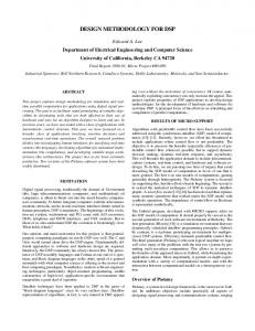
and the parameter vector X is de ned in Table 5. In addition, (NOx + HC)0, PM0 and BSFC0 are the emissions and fuel consumption target values, while W1 and W2 are weighting constants (safety factors). In order to establish proper targets for the optimization process, the engine was experimentally run in a baseline con guration with the standard EUI injection system, using operating parameter values taken from the operating map of the six cylinder production version of the Caterpillar 3400 Series engine (500 hp 3406E). Engine testing was performed at 1737 rev/min and 57% load. The test conditions for the EUI baseline engine tests were given in Table 4. Figure 2 is a plot of the measured PM emissions and BSFC vs. NOx+HC emissions for the range of injection timings evaluated during the EUI baseline tests. The PM vs. NOx+HC data exhibits a \best" emissions point at the +3.5 atdc timing (see box). The emissions levels at the +3.5 timing were used to calculate targets for the optimization. The NOx+HC emissions target for the present optimization was set to be 0.625 times the boxed point's NOx+HC level (i.e., 3.04 vs. the boxed point's 4.87 g/kW{hr). The target PM level was set at the boxed point's PM level (0.064 g/kW{hr). These levels were chosen because the six cylinder version of the SCOTE with parameters given in Table 4 is tuned to meet the 1998 US EPA NOx+HC emissions levels. Thus, if one were able to reduce the NOx+HC emissions levels to 0.625 times the original value and retain the present PM levels, then the engine should meet the proposed 2004 emissions levels, which requires a reduction of 0.625 for NOx+HC with respect to the 1998 regulations, while retaining the same PM level. Figure 2 also shows BSFC vs. NOx+HC. The data point corresponding to the \best" emissions point is boxed, and the target BSFC0 level was set to this level (256 g/kW{hr). Using these values for the emissions and BSFC targets in the previously stated merit function (with W1 = W2 = 1) 12

gives a concise goal which will reward strategies that are consistent with values that would meet the US EPA's 2004 emissions levels while maintaining a reasonable BSFC. While the rst two KIVA{GA runs and the experimental RSM optimization case employ the target values described above, the target values for a third KIVA{GA run, which includes a higher maximum EGR level (see Table 5), were chosen to be the 2004 EPA mandated emissions levels with weighting constants of W1 = W2 = 0:8. In addition, a lower BSFC0 target value of 215 g/kW{hr was used for this case. A summary of target values used in the present work is given in Table 6. As stated above, the one{dimensional gas{dynamics code of Zhu and Reitz (1999) was interfaced with KIVA{3V, which allows for simulations of the entire engine cycle. The one{dimensional code not only provides initial conditions for KIVA{3V at the time of intake valve closure (IVC), but also provides an estimate of work during the intake and exhaust strokes for use in the BSFC calculation. The computational mesh used in the present simulations is shown in Fig. 3. For computational eÆciency, a 60{degree sector of the combustion chamber is modeled due to the six{fold symmetry of the six{hole injector nozzle. Figures 4 and 5 show initial validation results from the present modeling methodology for the GA{Baseline case de ned in Table 4. It is clear that the model agrees reasonably well with the measured cylinder pressure and heat release rate. In addition, the engine{out soot and NOx levels agree well with the measured values (see Figs. 10 and 11). 5.4

Constraint Function

Durability constraints on the test engine include a maximum exhaust temperature Tex of 1023 K and a peak combustion pressure Pmax of approximately 15 MPa. In the present work, a \penalty function" approach was employed in order to inhibit convergence to an unphysical solution (i.e., one that violates the present constraints). For example, the peak pressure and exhaust temperature constraints are imposed by de ning a modi ed merit function f (X) given by 0

f (X) = f (X) (Pmax 0

15)2

(Tex

1023)2

(6)

where f (X) is given by Eqs. (2){(5) and =50.0, =0.5, but  = 0 if Pmax  15 MPa and = 0 if Tex  1023 K. The above approach was chosen since it penalizes designs based on how much the constraints are violated. This is important in the KIVA{GA optimization methodology since some 13

of the parameters from designs with slight constraint violations may be close to optimal. 5.5

Search Technique

The nal, and perhaps most important, element of the KIVA{GA methodology is the GA optimization technique described above. The KIVA{GA code is completely automated to simulate a GA generation (i.e., ve designs) in parallel. Once the ve simulations are completed, the genetic operators produce a new population and the process is repeated. 6

Results and Discussion

6.1

Computational Design Methodology Results

This section presents results from the KIVA{GA computational design methodology and compares them with the experimental RSM optimization results. In addition, \ultra{low" emissions are sought in the following section with a KIVA{GA run that includes a maximum EGR level of 50%. 6.1.1

Genetic Algorithm (KIVA{GA) Optimization

Figure 6 presents the maximum merit function f (X) vs. generation number for the rst KIVA{GA run. This optimization run includes approximately 250 full{cycle engine simulations, corresponding to about 12 days of continuous running on ve CPUs of an SGI Origin 2000 system. It is clear from Fig. 6 that the present methodology has found an optimum with a signi cantly higher merit function value compared to the GA{Baseline case (see also Table 8). A second KIVA{GA run was performed in order to demonstrate the repeatability and convergence of the design methodology. For the second run, KIVA{GA Run 2, a dierent random initial population was chosen while maintaining the same baseline case (i.e., step 1 of the GA). Figure 6 also shows maximum merit function vs. generation number for this case. While the second KIVA{GA run obtains more t solutions early on, a \local optimum" is apparently achieved which remains the most t design for many generations. This local optimum resides near the experimental RSM optimum in parameter space, as will be discussed further in a following section. However, by generation 100, KIVA{GA Run 2 has found a \best{ so{far" design with parameters very similar to the optimum of KIVA{GA Run 1, as shown also in Fig. 7. In this gure, factor levels have been normalized by the GA{Baseline values, and the absolute 0

14

values of each parameter are given above the bars. It was decided that the six optimum parameter values for KIVA{GA Runs 1 and 2 were suÆciently similar such that additional generations were not necessary in order to demonstrate convergence. Figures 8 and 9 present the predicted engine{out soot vs. NOx and BSFC vs. NOx points, respectively, for all of the approximately 250 simulation points of the KIVA{GA Run 1. It is clear from the gures that the optimum design results in signi cantly lower soot and NOx emissions compared to the baseline con guration. Furthermore, while the optimum point's BSFC is slightly higher than the baseline's value, it is still below the target value of 256 g/kW{hr. The increase in BSFC is attributed to the later injection timing (+4.6 atdc vs. +1 atdc of the GA{Baseline case). Figures 10 and 11 present NOx and soot, respectively, as functions of time for the baseline and optimum cases. As previously mentioned, a substantional reduction in both NOx and soot is achieved with, primarily, a higher EGR level, a more retarded injection timing and more fuel in the rst pulse of the split injection (see Fig. 7). 6.1.2

Comparison with Experiment

In order to validate the optimum point predicted by the KIVA{GA Run 1 case, engine experiments were run at the conditions given in Fig. 7 (grey bars). The combustion and emissions results are presented in Figs. 12{14. (It should be noted that due to hardware limitations, the fuel ow rate in the experiment had to be increased by approximately 8% in order to allow the injector to obtain 12% mass in the second pulse, as predicted in the simulation. As a result, the simulation was repeated at the GA{Optimum conditions with this 8% increase in fuel ow rate.) Both cylinder pressure and the soot and NOx emissions predicted by the simulation agree satisfactorialy well with the measured data, as seen in Figs. 12{14. Note that the experiment conducted at the GA{Optimum conditions resulted in a much lower NOx+HC level compared to the \best" emissions point of the EUI baseline (1.76 compared to 4.87 g/kW{hr) with very similar particulate and BSFC values to those predicted, providing evidence that the present method has found an optimum. 6.2

Comparison with Experimental RSM Optimization

The experimental RSM optimization methodology as described above was also used to explore the eect of the six engine input parameters on emissions and fuel consumption for the 1737 rev/min, 15

57% load operating point. A summary of the Response Surface Method steps is presented in Table 7. The process began with a fractional factorial experiment conducted around the starting point parameters given in Table 7. A gradient was next determined from a linear equation t to the experimental results, and a series of experiments were performed along the hyperline indicated by this gradient. The center point for the next factorial experiment was determined and is also given in Table 7 (i.e., the First Ascent column). A second ascent determined the center point for the third fractional factorial, and a third ascent established the point which is believed to be the optimum achieved by this method. Details of the RSM optimization process are given by Montgomery and Reitz (2000). Figures 15 and 16, which show soot vs. NOx+HC and BSFC vs. NOx+HC, respectively, present a graphical picture of the RSM process. Also included in these graphs is the EUI baseline data of Fig. 2 for reference. It is clear that the RSM{optimum results in signi cantly reduced NOx+HC emissions, together with improved soot and BSFC compared to the \best" emissions point (shown boxed) of the EUI baseline. The resulting RSM{optimum point was also simulated using the present KIVA code in order to further validate the present combustion modeling methodology. The resulting soot/NOx+HC and BSFC points are also included in Figs. 15 and 16 for comparison. The agreement between the measured and computed NOx+HC and BSFC is seen to be very good, while the soot is somewhat over{predicted by the model. For further comparison, the measured and predicted in{cylinder pressure and soot and NOx emissions are presented in Figs. 17 and 18, respectively. The good agreement between measurement and computation for the GA{Baseline (see Figs. 4, 5, 10 and 11), GA{Optimum (see Figs. 12{14) and the RSM{Optimum (see Figs. 15{18) suggests that the present model adequately predicts combustion and emissions over the entire range of engine input parameters and also serves to validate the present KIVA{GA optimization results. Figures 15 and 16 also include soot/NOx+HC and BSFC/NOx+HC points for the local optimum of KIVA{GA Run 2 (see Fig. 6). A comparison of design factors for the RSM{Optimum and GA Local Optimum cases are presented in Fig. 19. In this gure, factor levels have been normalized by the RSM{Optimum values, and the absolute values of each parameter are given above the bars. Interestingly, the local optimum of the KIVA{GA prediction appears to lie near the RSM{Optimum in parameter space. However, the somewhat increased EGR level and reduced injection pressure 16

are likely responsible for the decreased NOx+HC emissions, while the earlier injection timing and alternate split injection scheme are thought to result in the decreased soot emissions compared to the RSM{Optimum case. Furthermore, the advanced timing results in a slightly lower BSFC value, as shown in Fig. 16. The soot/NOx and BSFC/NOx points for the optimized condition predicted by KIVA{GA Run 1 are also shown in Figs. 15 and 16. It is important to note that while the GA{Optimum case results in lower soot and NOx emissions, resulting in a higher merit function value compared to the RSM{Optimum and GA Local Optimum cases, the predicted BSFC is higher than either of these cases (see Table 8). This implies that the present optimization techniques have found two regions of the present parameter space which result in signi cantly lower emissions compared to the EUI Baseline case. The RSM{Optimum/GA Local Optimum region has the added feature of a much lower BSFC value compared to the EUI baseline's best emissions point, while the GA{Optimum has even lower emissions but only a slightly lower BSFC value compared to the boxed point of the EUI baseline. 6.3

Toward Ultra{Low Emissions

Figures 20 and 21 present predicted engine{out soot vs. NOx and BSFC vs. NOx points, respectively, for KIVA{GA Run 3 (see Tables 5 and 6), which includes a maximum EGR level of 50% which is higher than was possible to achieve with the current engine installation. As in KIVA{GA Run 1, data from approximately 250 simulations are included in these gures. It is clear from Figs. 20 and 21 that the present methodology has once again found an optimum design with signi cantly lower soot and NOx emissions compared to the GA{Baseline case (also see Table 8). In addition, this optimum has the added feature of improved fuel consumption compared to the baseline case. It is important to note that it is not possible to be certain whether the point labeled \optimum" in Figs. 20 and 21 is in fact the global optimum since its value is not known. While experimental validation was available for the previous optimization cases (i.e., KIVA{GA Runs 1 and 2), it is not at this time available for the very high EGR levels used in this third optimization case. There are, however, a number of indications that the present optimum is in fact the global optimum, or is near the global optimum. First of all, Senecal (2000) has shown that the present GA performs extremely well for analytic test functions with many maxima. Furthermore, the repeatability and 17

convergence test presented above indicates that essentially the same optimum is achieved when the process is started with two dierent initial populations. Lastly, a majority of the points shown in Fig. 20 seem to follow a soot/NOx tradeo curve with the \optimum" point appearing visually to be the best compromise between soot, NOx and BSFC. In any case, the primary goal of a search technique for such a complex system is signi cant improvement and not necessarily the absolute best design point. The present design methodology has resulted in signi cant improvement with a 70% reduction in NOx, 50% reduction in soot (g/kg{fuel basis) and, simultaneously, improved fuel economy. A comparison of the design factors for the baseline and KIVA{GA Run 3 optimum designs is presented in Fig. 22. In this gure, factor levels have been normalized by the baseline values, and the absolute values of each parameter are given above the bars. As illustrated in the gure, the optimum con guration has a higher boost pressure and EGR level, a slightly advanced SOI, a shorter injection duration (i.e., a higher injection pressure), more mass in the rst injection pulse and a shorter dwell between injections. More details of this case are described by Senecal and Reitz (2000) where it is shown that the large NOx reduction is due to the fact that peak in{cylinder gas temperatures are reduced signi cantly with the high EGR level. While the focus thus far has been on the optimum design, it is also of interest to examine the extreme soot/NOx points in Fig. 20. Again, the design factors for the extreme high soot/low NOx point (see Fig. 20, arrows) are given in Fig. 23. As in Fig. 22, the design factors have been normalized by the baseline values and the absolute values are given above the bars. It is interesting to note that the boost pressure and EGR values are essentially identical to those of the optimum design. On the other hand, this design includes a very retarded injection timing (about +7 deg. atdc) and a longer injection duration (corresponding to a lower injection pressure of about 106 MPa). Retarded injection timings and low injection pressures are traditionally known to result in relatively high soot and low NOx. Note that the predicted NOx level of this point is as low as 0.2 g/kW{hr (compared to the minumum NOx level of 0.7 g/kW{hr when a maximum EGR level of 25% was used, see Fig. 8). However, due to the high soot, engine operation approaching this condition might only be possible with use of triple or quadruple injections (Montgomery and Reitz 1996), low sooting fuels (e.g., oxygenates (Choi and Reitz 1999)) or with eective particulate traps. 18

7

Summary and Conclusions

This work establishes a computational methodology for engine design using multi{dimensional spray and combustion modeling in conjunction with experimental validation. The KIVA{GA code incorporates improved physical submodels in the KIVA{3V CFD code coupled with a one{dimensional gas dynamics code for full cycle engine calculations within the framework of a GA optimization technique. The GA eÆciently determined a set of engine input parameters resulting in signi cantly lower soot and NOx emissions compared to the baseline case. The optimum case also demonstrated improved fuel consumption compared to the baseline. The present methodology provides a useful tool for engine designers investigating the eects of a large number of input parameters on emissions and performance. Results from the experimental Response Surface Method were used to aid in the formulation and validation of the present design methodology. This RSM approach found a similar optimum with improved emissions and fuel consumption compared to the baseline case. The success of both techniques, experimental and computational, suggests that one method could be used to provide an \initial guess" for the other in future optimization studies. 8

Acknowledgements

This work was supported by the Army Research OÆce under Grant No. DAAHL03{92{0122, Caterpillar Inc. and DOE/Sandia labs. The authors would like to thank K. Richards, Dr. D. L. Carroll and Dr. Y. Zhu for helpful comments and Matt Thiel and Craig Marriott for providing the experimental data in Figs. 12{14. References

[1] Aes, H., Trigui, N., Smith, D. and Griaznov, V., \Shape Optimization of IC Engine Ports and Chambers," SAE 980127, 1998. [2] Amsden, A. A., \KIVA{3V: A Block{Structured KIVA Program for Engines with Vertical or Canted Valves," Los Alamos National Laboratory Report No. LA-13313-MS, 1997. 19

[3] Bowman, C. T., \Kinetics of Pollutant Formation and Destruction in Combustion," Prog. Energy Combust. Sci., 1, 33, 1975. [4] Box, G. E. P. and Draper, N. R., \Empirical Model{Building and Response Surfaces," Wiley, ISBN 0{471{81033{9, 1986. [5] Carroll, D. L., \Chemical Laser Modeling with Genetic Algorithms," AIAA Journal, 34, 338, 1996a. [6] Carroll, D. L., \Genetic Algorithms and Optimizing Chemical Oxygen{Iodine Lasers," Developments in Theoretical and Applied Mechanics, 18, 411, 1996b. [7] Chan, M., Das, S. and Reitz, R. D., \Modeling of Multiple Injection and EGR Eects on Diesel Engine Emissions," SAE 972864, 1997. [8] Choi, C. Y. and Reitz, R. D., \An Experimental Study on the Eects of Oxygenated Fuel Blends and Multiple Injection Strategies on DI Diesel Engine Emissions," Fuel, 78, 1303, 1999. [9] Coello Coello, C. A., Christiansen, A. D. and Santos Hernandez, F., \A Simple Genetic Algorithm for the Design of Reinforced Concrete Beams," Engineering with Computers, 13, 185, 1997. [10] Edwards, S. P., Pilley, A. D., Michon, S. and Fournier, G., \The Optimization of Common Rail FIE Equipped Engines Through the use of Statistical Experimental Design, Mathematical Modelling and Genetic Algorithms," SAE 970346, 1997. [11] Gibson, D. H., Shinogle, R. D. and Moncelle, M. E., \Meeting the Customer's Needs { De ning the Next Generation Electronically Controlled Unit Injector Concept for Heavy Duty Diesel Engines," SAE 961285, 1996. [12] Halstead, M., Kirsh, L. and Quinn, C., \The Autoignition of Hydrocarbon Fuels at High Temperatures and Pressures { Fitting of a Mathematical Model," Combust. Flame, 30, 45, 1977. [13] Han, Z. and Reitz, R. D., \Turbulence Modeling of Internal Combustion Engines Using RNG k{ Models," Combust. Sci. and Tech., 106, 267, 1995. [14] Han, Z., Uludogan, A., Hampson, G. J. and Reitz, R. D., \Mechanism of Soot and NOx Emission Reduction Using Multiple{Injection in a Diesel Engine," SAE 960633, 1996. 20

[15] Han, Z. and Reitz, R. D., \A Temperature Wall Function Formulation for Variable{Density Turbulence Flows with Application to Engine Convective Heat Transfer Modeling," Int. J. of Heat and Mass Transfer, 40, 613, 1997. [16] Heywood, J. B., \Internal Combustion Engine Fundamentals", McGraw{Hill, Inc., ISBN 0{07{ 028637{X, 1988. [17] Hikosaka, N., \A View of the Future of Automotive Diesel Engines," SAE 972682, 1997. [18] Hiroyasu, H. and Kadota, T., \Models for Combustion and Formation of Nitric Oxide and Soot in DI Diesel Engines," SAE 760129, 1976. [19] Kong, S.-C., Han, Z. and Reitz, R. D., \The Development and Application of a Diesel Ignition and Combustion Model for Multidimensional Engine Simulation," SAE 950278, 1995. [20] Krishnakumar, K., \Micro{Genetic Algorithms for Stationary and Non{Stationary Function Optimization," SPIE 1196, Intelligent Control and Adaptive Systems, 1989. [21] Montgomery, D. T. and Reitz, R. D., \Six{Mode Cycle Evaluation of the Eect of EGR and Multiple Injections on Particulate and NOx Emissions from a D. I. Diesel Engine," SAE 960316, 1996. [22] Montgomery, D. T., Ph.D. Thesis (in preparation), University of Wisconsin{Madison, 2000. [23] Montgomery, D. T. and Reitz, R. D., \Optimization of Heavy{Duty Diesel Engine Operating Parameters using a Response Surface Method," submitted to SAE, 2000. [24] Nagle, J. and Strickland{Constable, R. F., \Oxidation of Carbon between 1000{2000 C," Proc. of the Fifth Carbon Conf., 1, 154, 1962. [25] Patterson, M. A., Kong, S.-C., Hampson, G. J. and Reitz, R. D., \Modeling the Eects of Fuel Injection Characteristics on Diesel Engine Soot and NOx Emissions," SAE 940523, 1994. [26] Pierpont, D. A. and Reitz, R. D., \Eects of Injection Pressure and Nozzle Geometry on D. I. Diesel Emissions and Performance," SAE 950604, 1995. 21

[27] Pilley, A. D., Beaumont, A. J., Robinson, D. R. and Mowll, D., \Design of Experiments for Optimization of Engines to Meet Future Emissions Targets," 27th Int. Symposium on Automotive Technology and Automation, ISATA Paper 94EN014, 1994. [28] Rao, S. S., \Optimization { Theory and Applications," Wiley Eastern, ISBN 0{85226{756{8, 1978. [29] Rutland, C. J., Eckhause, J., Hampson, G., Hessel, R., Kong, S., Patterson, M., Pierpont, D., Sweetland, P., Tow T. and Reitz, R. D., \Toward Predictive Modeling of Diesel Engine Intake Flow, Combustion, and Emissions," SAE 941897, 1994. [30] Sarre, C., Kong, S.-C. and Reitz, R. D., \Modeling the Eects of Injector Nozzle Geometry on Diesel Sprays," SAE 1999{01{0912, 1999. [31] Senecal, P. K., Uludogan, A. and Reitz, R. D., \Development of Novel Direct{Injection Diesel Engine Combustion Chamber Designs using Computational Fluid Dynamics," SAE 971594, 1997. [32] Senecal, P. K., Ph.D. Thesis (in preparation), University of Wisconsin{Madison, 2000. [33] Senecal, P. K. and Reitz, R. D., \Simultaneous Reduction of Diesel Engine Emissions and Fuel Consumption using Genetic Algorithms and Multi{Dimensional Spray and Combustion Modeling," submitted to SAE, 2000. [34] Tanin, K. V., Wickman, D. D., Montgomery, D. T., Das, S. and Reitz, R. D., \The In uence of Boost Pressure on Emissions and Fuel Consumption of a Heavy{Duty Single{Cylinder D. I. Diesel Engine," SAE 1999{01{0840, 1999. [35] Wickman, D. D., Tanin, K. V., Senecal, P. K., Reitz, R. D., Gebert, K., Barkhimer, R. L. and Beck, N. J., \Methods and Results from the Development of a 2600 Bar Diesel Fuel Injection System," SAE 2000{01{0947, 2000. [36] Zhu, Y. and Reitz, R. D., \A 1{D Gas Dynamics Code for Subsonic and Supersonic Flows Applied to Predict EGR Levels in a Heavy{Duty Diesel Engine," Int. J. of Vehicle Design, 22, 227, 1999. 22

Table 1: Engine speci cations. Engine Type

Caterpillar SCOTE (single{cylinder oil test engine) { direct injection { 4 valve Bore  Stroke 137.2 mm  165.1 mm Compression Ratio 15.6:1 Displacement 2.44 liters Combustion Chamber Quiescent Piston Articulated Steel/Aluminum Mexican Hat Sharp Edge Crater

23

Table 2: EUI and NGEUI speci cations. Injector Injection Pressure Number of Nozzle Holes Nozzle Hole Diameter Included Spray Angle EUI Up to 190 MPa 6 0.214 mm 130 deg. NGEUI Up to 210 MPa 6 0.188 mm 125 deg.

24

Table 3: Emissions instrumentation. NOx THC CO2 PM

Chemiluminescent Analyzer/Thermo Environmental Instruments Inc., Model 10S Flame Ionization Detector/Gow{Mac, Model 23{500 Infrared Gas Analyzer/Horiba, Model VIA{510 Full Dilution Tunnel (EPA 40CFR Design)

25

Table 4: Engine parameters and operating conditions for the baseline engine cases. Parameter Engine Speed % of Maximum Load Fuel Rate Intake Temperature Intake Pressure Exhaust Pressure Injection Pressure Start of Injection EGR Level Injection scheme

GA{Baseline (NGEUI) 1737 rpm 57 6.97 kg/hr 305 K 184 kPa 181 kPa 150 MPa +1 deg. atdc 12% 68(10.5)32 split

26

EUI Baseline 1737 rpm 57 6.97 kg/hr 305 K 184 kPa 181 kPa 150 MPa -3.5 to +5.5 deg. 0% single

Table 5: Design factors and ranges considered. Boost Pressure EGR Level

165 ! 284 kPa 0 ! 25% (KIVA{GA Runs 1 and 2) 0 ! 50% (KIVA{GA Run 3) Start of Injection -10 ! +10 deg. atdc Injection Duration
inj 20.5 ! 29.0 deg. (Injection Pressure Pinj ) (100 ! 200 MPa) Mass in First Pulse 10 ! 90 % Dwell Between Pulses 5 ! 15 deg.

27

Table 6: Summary of KIVA{GA and RSM optimization cases. Case Merit function Target Values (g/kW{hr) W1 W2 KIVA{GA Run 1 & 2, f (X) = 1000=(R12 + R22 + R3) (NOx + HC)0 = 3:04 1.0 1.0 RSM PM0 = 0:064 BSFC0 = 256 KIVA{GA Run 3 f (X) = 1000=(R12 + R22 + R3 ) (NOx + HC)0 = 3:35 0.8 0.8 PM0 = 0:13 BSFC0 = 215

28

Table 7: Summary of experimental RSM optimization. Parameter Boost Pressure EGR Level Start of Injection Injection Pressure Mass in First Pulse Dwell Between Pulses

Start Point (1) 181 kPa 20.5% -0.5 deg. atdc 150 MPa 60% 10 deg.

First Ascent (2) 181 kPa 19.5% +0.5 deg. atdc 161.5 MPa 72% 10 deg.

29

Second Ascent (3) 169 kPa 19.3% -2.0 deg. atdc 180 MPa 55% 10 deg.

Optimized Condition (4) 169 kPa 20% -2.5 deg. atdc 180 MPa 55% 9.2 deg.

Table 8: Summary of KIVA{GA and experimental RSM optimization results. Note that the calculation of the merit function for the rst six cases is dierent from the calculation for the last two cases according to the target values given in Table 6. Case GA{Baseline EUI Baseline Best Point RSM{Optimum GA Local Optimum Optimum, KIVA{GA Run 2 Optimum, KIVA{GA Run 1 GA{Baseline Optimum, KIVA{GA Run 3

soot (g/kW{hr) 0.124 0.064 0.045 0.032 0.029 0.030 0.124 0.042

NOx+HC (g/kW{hr) 3.75 4.87 2.31 1.89 1.68 1.32 3.75 1.01

30

BSFC (g/kW{hr) 240.5 256.0 238.6 236.6 245.9 248.9 240.5 212.1

Merit 161.6 218.9 499.0 637.3 681.3 722.5 222.3 774.2

Figure 1: Engine laboratory setup.

31

0.160

280.0

270.0 0.120

−3.5

PM (g/kW−hr)

+2.5 0.080

250.0

+5.5 −0.5 +3.5

+1.5

BSFC (g/kW−hr)

260.0

240.0

0.040 230.0

0.000 4.0

4.5

5.0 5.5 6.0 NOx + HC (g/kW−hr)

6.5

220.0 7.0

Figure 2: Measured EUI baseline engine emissions and fuel consumption.

32

Figure 3: Computational mesh for the Caterpillar engine at TDC. One{sixth of the domain is used because of symmetry.

33

10.0 Measured Computed

Pressure (MPa)

8.0

6.0

4.0

2.0

0.0 −50 −40 −30 −20 −10 0 10 20 crank angle (deg. atdc)

30

40

50

60

Figure 4: Comparison of measured (Montgomery and Reitz 2000) and computed cylinder pressure for the GA{Baseline case (see Table 4).

34

0.05

Normalized Heat Release Rate (1/deg.)

Measured Computed 0.04

0.03

0.02

0.01

0.00

0

10

20 30 40 crank angle (deg. atdc)

50

60

Figure 5: Comparison of measured (Montgomery and Reitz 2000) and computed heat release rate for the GA{Baseline case (see Table 4).

35

900.0 KIVA−GA Run 1 KIVA−GA Run 2

800.0

Maximum Merit Function

700.0 600.0 Local Optimum 500.0 400.0 300.0 Baseline 200.0 100.0 0.0 0.0

20.0

40.0 60.0 Generation Number

80.0

100.0

Figure 6: Maximum merit function value vs. generation number for KIVA{GA Runs 1 and 2 demonstrating convergence. Arrows indicate the GA{Baseline value and \local optimum" merit function value for KIVA{GA Run 2.

36

5.0 +4.6 +4.2

4.0

GA−Baseline Optimum, KIVA−GA Run 1 Optimum, KIVA−GA Run 2

x/xbase

3.0

2.0

22.6 21.0 88 88

1.0

0.0

184 187 187

Boost

12

EGR

+1

23.5 23 23

SOI

∆Θinj

68

% Mass

13.5 12.7 10.5

Dwell

Figure 7: Comparison of design factors for the GA{Baseline and optimum cases for KIVA{GA Runs 1 and 2. Actual values of each parameter (in units consistent with Table 5) are given above the bars.

37

0.60

soot (g/kW−hr)

0.45

0.30

Baseline 0.15

0.00 0.0 2.0 Optimum

4.0

6.0 8.0 NOx (g/kW−hr)

10.0

12.0

Figure 8: Soot vs. NOx data from KIVA{GA Run 1 for all simulation cases including the GA{ Baseline and optimum.

38

340.0 320.0

BSFC (g/kW−hr)

300.0 280.0 Baseline

260.0 240.0 220.0

Optimum

200.0 180.0 0.0

2.0

4.0

6.0 8.0 NOx (g/kW−hr)

10.0

12.0

Figure 9: BSFC vs. NOx data from KIVA{GA Run 1 for all simulation cases including the GA{ Baseline and optimum.

39

20.0

NOx (g/kg−fuel)

16.0

GA−Baseline (Measured) GA−Baseline (Computed) Optimum, KIVA−GA Run 1 Optimum, KIVA−GA Run 3

12.0

8.0

4.0

0.0 0.0

20.0

40.0

60.0 80.0 100.0 crank angle (deg. atdc)

120.0

140.0

Figure 10: Comparison of measured and predicted NOx for the GA{Baseline case and optimum cases for KIVA{GA Runs 1 and 3.

40

5.0 GA−Baseline (Measured) GA−Baseline (Computed) Optimum, KIVA−GA Run 1 Optimum, KIVA−GA Run 3

soot (g/kg−fuel)

4.0

3.0

2.0

1.0

0.0 0.0

20.0

40.0

60.0 80.0 100.0 crank angle (deg. atdc)

120.0

140.0

Figure 11: Comparison of measured and predicted soot for the GA{Baseline case and optimum cases for KIVA{GA Runs 1 and 3.

41

12.0 Measured Computed 10.0

Pressure (MPa)

8.0

6.0

4.0

2.0

0.0 −40.0

−20.0

0.0 20.0 crank angle (deg. atdc)

40.0

60.0

Figure 12: Comparison of measured and predicted in{cylinder pressure for the GA{optimum design.

42

10.0 Measured Computed

soot (g/kg−fuel)

8.0

6.0

4.0

2.0

0.0 0.0

20.0

40.0

60.0 80.0 100.0 crank angle (deg. atdc)

120.0

140.0

Figure 13: Comparison of measured and predicted soot for the GA{optimum design.

43

10.0 Measured Computed

NOx (g/kg−fuel)

8.0

6.0

4.0

2.0

0.0 0.0

20.0

40.0

60.0 80.0 100.0 crank angle (deg. atdc)

120.0

140.0

Figure 14: Comparison of measured and predicted NOx for the GA{optimum design.

44

0.25

soot (g/kW−hr)

0.20

0.15

EUI Baseline RSM − Optimization Start Point RSM − After First Ascent RSM − After Second Ascent RSM − Optimized Condition KIVA Prediction at RSM Optimum GA − Local Optimum GA − Optimized Condition 1

0.10

2

3 4

0.05

0.00 0.0

2.0

4.0 NOx+HC (g/kW−hr)

6.0

8.0

Figure 15: Comparison of experimental (RSM) and computational (KIVA{GA) optimization emissions results. Numbers next to the RSM points correspond to the numbers given in Table 7.

45

320.0

BSFC (g/kW−hr)

300.0

280.0

EUI Baseline RSM − Optimization Start Point RSM − After First Ascent RSM − After Second Ascent RSM − Optimized Condition KIVA Prediction at RSM Optimum GA − Local Optimum GA − Optimized Condition

260.0 1 2 4 3

240.0

220.0 0.0

2.0

4.0 NOx+HC (g/kW−hr)

6.0

8.0

Figure 16: Comparison of experimental (RSM) and computational (KIVA{GA) optimization fuel consumption results. Numbers next to the RSM points correspond to the numbers given in Table 7.

46

10.0 Measured Computed

Pressure (MPa)

8.0

6.0

4.0

2.0

0.0 −40.0

−20.0

0.0 20.0 crank angle (deg. atdc)

40.0

60.0

Figure 17: Comparison of measured and KIVA predicted in{cylinder pressure at the RSM{optimum design.

47

5.0

14.0 12.0

NOx (measured) NOx (computed)

soot (measured) soot (computed) 4.0

3.0

8.0 6.0

2.0

soot (g/kg−fuel)

NOx (g/kg−fuel)

10.0

4.0 1.0 2.0 0.0 0.0

20.0

40.0

60.0 80.0 100.0 crank angle (deg. atdc)

120.0

0.0 140.0

Figure 18: Comparison of measured (engine{out) and KIVA predicted soot and NOx at the RSM{ optimum design.

48

2.0 RSM − Optimum GA − Local Optimum 1.5

−3.6

x/xRSM−Optimum

24.2

1.0

169 169.4 20

180

−2.5

55

9.2 8.2

160 44

0.5

0.0

Boost

EGR

SOI

Pinj

% Mass

Dwell

Figure 19: Comparison of design factors for the RSM{Optimum and GA Local Optimum cases. Actual values of each parameter (in units consistent with Table 5) are given above the bars.

49

0.60 High soot/Low NOx 0.50

soot (g/kW−hr)

0.40

0.30

0.20 Baseline

High NOx/Low soot

0.10

0.00 0.0 2.0 Optimum

4.0

6.0 8.0 NOx (g/kW−hr)

10.0

12.0

Figure 20: Soot vs. NOx data from KIVA{GA Run 3 for all simulation cases including the GA{ Baseline and optimum.

50

350.0 High soot/Low NOx

BSFC (g/kW−hr)

300.0

Baseline 250.0

200.0 Optimum High NOx/Low soot 150.0 0.0

2.0

4.0

6.0 8.0 NOx (g/kW−hr)

10.0

12.0

Figure 21: BSFC vs. NOx data from KIVA{GA Run 3 for all simulation cases including the GA{ Baseline and optimum.

51

4.5 GA−Baseline Optimum, KIVA−GA Run 3

46

3.5

x/xbase

2.5

1.5

230 184

12

23.5 21.2

+1

68

80

10.5 7.2

0.5

−0.5 −1

−1.5

Boost

EGR

SOI

∆Θinj

% Mass

Dwell

Figure 22: Comparison of design factors for the GA{Baseline and optimum case for KIVA{GA Run 3. Actual values of each parameter (in units consistent with Table 5) are given above the bars.

52

8.0 Baseline High soot/Low NOx

+7.2

7.0 6.0

x/xbase

5.0 47

4.0 3.0 2.0 1.0 0.0

184

227

Boost

12

EGR

23.5

+1

SOI

28

∆Θinj

68

53

% Mass

10.5

7.8

Dwell

Figure 23: Comparison of design factors for the GA{Baseline and high soot/low NOx cases. Actual values of each parameter are given above the bars.

53